SciPy in Python

Here are a few useful SciPy sample codes showcasing different aspects of the library, including optimization, integration, interpolation, and signal processing.

1. Optimization: Minimizing a Function

This example demonstrates how to minimize a mathematical function using scipy.optimize.

1
2
3
4
5
6
7
8
9
10
11
12
13
14
15

import numpy as np
from scipy.optimize import minimize

# Define a function to minimize
def objective_function(x):
    return x**2 + 10*np.sin(x)

# Initial guess
x0 = 2.0

# Perform the minimization
result = minimize(objective_function, x0, method='BFGS')

print("Minimum value of the function:", result.fun)
print("Value of x that minimizes the function:", result.x)

[Output]

Minimum value of the function: 8.31558557947746
Value of x that minimizes the function: [3.83746713]

2. Integration: Calculating the Area Under a Curve

This example shows how to calculate the definite integral of a function using scipy.integrate.quad.

1
2
3
4
5
6
7
8
9
10

from scipy.integrate import quad

# Define a function to integrate
def integrand(x):
    return np.exp(-x**2)

# Compute the integral from 0 to infinity
result, error = quad(integrand, 0, np.inf)

print("Integral result:", result)

[Output]

Integral result: 0.8862269254527579

3. Interpolation: Interpolating Data Points

This example demonstrates how to interpolate data points using scipy.interpolate.interp1d.

1
2
3
4
5
6
7
8
9
10
11
12
13
14
15
16
17
18
19
20

import numpy as np
import matplotlib.pyplot as plt
from scipy.interpolate import interp1d

# Sample data points
x = np.linspace(0, 10, 10)
y = np.sin(x)

# Create an interpolation function
f = interp1d(x, y, kind='cubic')

# Generate new x values and interpolate
x_new = np.linspace(0, 10, 100)
y_new = f(x_new)

# Plot the results
plt.plot(x, y, 'o', label='Data points')
plt.plot(x_new, y_new, '-', label='Cubic interpolation')
plt.legend()
plt.show()

[Output]

4. Signal Processing: Filtering a Signal

This example shows how to apply a low-pass filter to a noisy signal using scipy.signal.

1
2
3
4
5
6
7
8
9
10
11
12
13
14
15
16
17
18
19
20
21
22
23
24
25
26
27
28
29
30
31
32
33
34

import numpy as np
import matplotlib.pyplot as plt
from scipy.signal import butter, lfilter

# Generate a noisy signal
np.random.seed(0)
t = np.linspace(0, 1, 500, endpoint=False)
signal = np.sin(2 * np.pi * 7 * t) + 0.5 * np.random.randn(500)

# Design a low-pass filter
def butter_lowpass(cutoff, fs, order=5):
    nyquist = 0.5 * fs
    normal_cutoff = cutoff / nyquist
    b, a = butter(order, normal_cutoff, btype='low', analog=False)
    return b, a

# Apply the filter to the signal
def lowpass_filter(data, cutoff, fs, order=5):
    b, a = butter_lowpass(cutoff, fs, order=order)
    y = lfilter(b, a, data)
    return y

# Parameters
cutoff = 3.5  # Desired cutoff frequency of the filter, Hz
fs = 50.0     # Sample rate, Hz

# Filter the signal
filtered_signal = lowpass_filter(signal, cutoff, fs)

# Plot the results
plt.plot(t, signal, label='Noisy signal')
plt.plot(t, filtered_signal, label='Filtered signal', linewidth=2)
plt.legend()
plt.show()

[Output]

These examples provide a glimpse of the powerful tools available in SciPy for scientific computing, including optimization, integration, interpolation, and signal processing.

PuLP in Python

PuLP is a Python library used for linear programming (LP) and mixed-integer linear programming (MILP).

It allows you to define and solve optimization problems where you want to minimize or maximize a linear objective function subject to linear constraints.

Installation

First, you need to install PuLP. You can do this using pip:

1

pip install pulp

Basic Usage of PuLP

Here’s a step-by-step guide to solving a simple linear programming problem with PuLP.

Example Problem:

Suppose you are a factory manager and you want to determine the optimal number of products $A$ and $B$ to produce to maximize your profit.
Each product requires a certain amount of resources (time, materials) and yields a certain profit.

• Objective: Maximize profit.
• Constraints:
  • You have $100$ units of material.
  • You have $80$ hours of labor.
  • Product $A$ requires $4$ units of material and $2$ hours of labor.
  • Product $B$ requires $3$ units of material and $5$ hours of labor.
• Profit:
  • Product $A$ gives $20 profit per unit.
  • Product $B$ gives $25 profit per unit.

Step-by-Step Implementation

1
2
3
4
5
6
7
8
9
10
11
12
13
14
15
16
17
18
19
20
21
22
23
24
25
26
27
28
29
30

import pulp

# Step 1: Define the problem
# Create a maximization problem
problem = pulp.LpProblem("Maximize_Profit", pulp.LpMaximize)

# Step 2: Define the decision variables
# Let x be the number of product A to produce, y be the number of product B to produce
x = pulp.LpVariable('x', lowBound=0, cat='Continuous')
y = pulp.LpVariable('y', lowBound=0, cat='Continuous')

# Step 3: Define the objective function
# Objective function: Maximize 20x + 25y
problem += 20*x + 25*y, "Profit"

# Step 4: Define the constraints
# Constraint 1: 4x + 3y <= 100 (Material constraint)
problem += 4*x + 3*y <= 100, "Material"

# Constraint 2: 2x + 5y <= 80 (Labor constraint)
problem += 2*x + 5*y <= 80, "Labor"

# Step 5: Solve the problem
problem.solve()

# Step 6: Display the results
print("Status:", pulp.LpStatus[problem.status])
print("Optimal number of product A to produce:", pulp.value(x))
print("Optimal number of product B to produce:", pulp.value(y))
print("Maximum Profit:", pulp.value(problem.objective))

Explanation of the Code:

1. Define the Problem: We create a linear programming problem with the objective to maximize profit.
2. Decision Variables: We define the decision variables x and y for the number of products A and B to produce.
   These variables are continuous and non-negative.
3. Objective Function: We define the objective function to maximize, which is the total profit: 20*x + 25*y.
4. Constraints: We add constraints based on the available resources:
   • Material constraint: 4*x + 3*y <= 100
   • Labor constraint: 2*x + 5*y <= 80
5. Solve the Problem: We solve the linear programming problem using PuLP’s solve method.
6. Display the Results: We print the optimal values of x and y, and the maximum profit.

Interpretation of Output:

Output

1
2
3
4

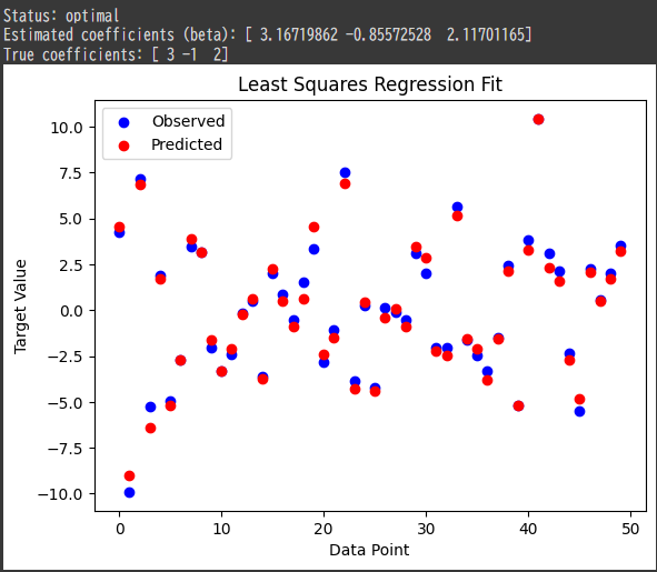
Status: Optimal
Optimal number of product A to produce: 18.571429
Optimal number of product B to produce: 8.5714286
Maximum Profit: 585.714295

Interpretation

• The optimal solution is to produce $18.5$ units of product A and $8.57$ units of product B, which yields a maximum profit of $585.71.

This is a basic example of using PuLP in Python.

The library is powerful and can handle more complex constraints, variables, and objectives, including mixed-integer programming.

Altair

Here’s a advanced and useful sample code using Altair, which demonstrates how to create a layered chart with interactivity, such as tooltips and selection, along with custom encoding:

1
2
3
4
5
6
7
8
9
10
11
12
13
14
15
16
17
18
19
20
21
22
23
24
25
26
27
28
29
30
31
32
33
34

import altair as alt
from vega_datasets import data

# Load dataset
source = data.cars()

# Define a brush selection
brush = alt.selection(type='interval')

# Base chart with a scatter plot
base = alt.Chart(source).mark_point().encode(
    x='Horsepower:Q',
    y='Miles_per_Gallon:Q',
    color=alt.condition(brush, 'Origin:N', alt.value('lightgray')),
    tooltip=['Name:N', 'Origin:N', 'Horsepower:Q', 'Miles_per_Gallon:Q']
).properties(
    width=600,
    height=400
).add_selection(
    brush
)

# Layer a bar chart on top that shows the distribution of 'Origin' for selected points
bars = alt.Chart(source).mark_bar().encode(
    x='count():Q',
    y='Origin:N',
    color='Origin:N'
).transform_filter(
    brush
)

# Combine the scatter plot and the bar chart
chart = base & bars
chart

Result

Explanation

• Brush Selection:
  An interactive selection that allows users to drag over the scatter plot to select a region.
• Scatter Plot:
  A basic plot where points are colored by their origin, and the color changes based on the selection.
• Bar Chart:
  Shows the distribution of car origins, updated based on the selection made in the scatter plot.
• Interactivity:
  Tooltips provide detailed information when hovering over the points, and the chart updates dynamically based on the user’s selection.

This example combines interactivity with advanced encoding and layout, making it useful for exploratory data analysis.

Altairを使用してPythonで複雑なグラフを作成する例を紹介します。

以下のコードでは、サンプルデータを作成し、複数のデータ系列を組み合わせた複雑な可視化を行います。

この例では、散布図と折れ線グラフを組み合わせたマルチレイヤーグラフを描きます。

1
2
3
4
5
6
7
8
9
10
11
12
13
14
15
16
17
18
19
20
21
22
23
24
25
26
27
28
29
30
31
32
33
34

import altair as alt
import pandas as pd
import numpy as np

# サンプルデータの作成
np.random.seed(0)
x = np.linspace(0, 100, 100)
y1 = np.sin(x / 10) + np.random.normal(0, 0.1, 100)
y2 = np.cos(x / 10) + np.random.normal(0, 0.1, 100)
category = np.random.choice(['A', 'B', 'C'], 100)

df = pd.DataFrame({'x': x, 'y1': y1, 'y2': y2, 'category': category})

# 散布図の作成
scatter = alt.Chart(df).mark_point().encode(
    x='x',
    y='y1',
    color='category',
    tooltip=['x', 'y1', 'category']
).properties(
    title='Scatter Plot with Line Chart Overlay'
)

# 折れ線グラフの作成
line = alt.Chart(df).mark_line(color='red').encode(
    x='x',
    y='y2'
)

# 散布図と折れ線グラフのオーバーレイ
combined_chart = scatter + line

# グラフの表示
combined_chart.show()

コードの説明

1. データの作成:
   numpyを使用して、$100$点のデータを生成しています。
   y1はノイズの入ったサイン波、y2はノイズの入ったコサイン波です。
   また、categoryはランダムに割り当てたカテゴリです。

2. 散布図の作成:
   alt.Chart(df).mark_point()で散布図を作成し、x, y1, categoryでデータをエンコードしています。

3. 折れ線グラフの作成:
   alt.Chart(df).mark_line(color='red')で折れ線グラフを作成し、x, y2でデータをエンコードしています。

4. グラフのオーバーレイ:
   scatter + lineで、散布図と折れ線グラフをオーバーレイして複合グラフを作成しています。

5. グラフの表示: combined_chart.show()でグラフを表示します。

[実行結果]

Altairを使用することで、簡単に複雑な可視化を作成できます。

このコードをGoogle Colabなどの環境で実行すると、インタラクティブなグラフが表示されます。

グラフ作成 Altair

Altairを使った簡単なグラフ作成のサンプルコードを紹介します。

Altairは宣言型で直感的にグラフを描けるため、データの視覚化が非常に簡単です。

以下のサンプルでは、Altairを使って基本的な散布図を作成します。

サンプルコード: Altairでの散布図作成

1
2
3
4
5
6
7
8
9
10
11
12
13
14
15
16
17
18
19
20
21
22
23

!pip install altair_viewer
import altair as alt
import pandas as pd

# サンプルデータの作成
data = pd.DataFrame({
    'x': [1, 2, 3, 4, 5],
    'y': [2, 3, 7, 6, 9],
    'category': ['A', 'A', 'B', 'B', 'C']
})

# Altairで散布図を作成
chart = alt.Chart(data).mark_circle(size=60).encode(
    x='x',
    y='y',
    color='category',  # カテゴリーに基づく色分け
    tooltip=['x', 'y', 'category']  # ホバー時に表示されるデータ
).properties(
    title='Simple Scatter Plot with Altair'
)

# グラフを表示
chart.show()

コードの解説

1. ライブラリのインポート:

   • import altair as alt: Altairライブラリをインポートします。
   • import pandas as pd: サンプルデータを作成するためにPandasをインポートします。

2. データの作成:

   • Pandasのデータフレームとしてデータを作成します。
     このデータにはx軸、y軸の値と、各点のcategory情報が含まれています。

3. Altairでの散布図作成:

   • alt.Chart(data): データフレームをAltairのチャートオブジェクトに変換します。
   • mark_circle(size=60): 円形のマークを使用して、各データポイントをプロットします。
   • encode: プロットの設定を行います。
     • x='x': x軸の値を設定。
     • y='y': y軸の値を設定。
     • color='category': カテゴリーごとに色を分けます。
     • tooltip=['x', 'y', 'category']: ホバー時に表示するデータの情報を設定します。
   • properties: グラフのタイトルやその他のプロパティを設定します。

4. グラフの表示:

   • chart.show(): グラフを表示します（Jupyter Notebookを使っている場合はchartとするだけで表示されます）。

実行結果

このコードを実行すると、カテゴリーごとに色分けされた散布図が表示されます。

各データポイントにマウスをホバーすると、ツールチップに$x$, $y$の値とカテゴリーが表示されます。

Altairは、簡単なコードでインタラクティブなグラフを作成できる強力なツールです。

さらに複雑なグラフも、同様の構文で簡単に作成できます。

最適化問題 SciPy

SciPyを用いて複雑な最適化問題を解き、その結果をグラフ化する例を示します。

以下では、非線形の目的関数と制約条件を持つ最適化問題を設定します。

問題設定

目的関数:
$$
f(x) = (x_0 - 2)^2 + (x_1 - 3)^2 + \cos(x_0 \cdot x_1)
$$

制約条件:

1. 非線形等式制約:
   $$
   g_1(x) = x_0^2 + x_1^2 - 4 = 0
   $$

2. 非線形不等式制約:
   $$
   g_2(x) = x_0 \cdot x_1 - 1 \geq 0
   $$

初期推定値として$ ( x_0 = 1 ), ( x_1 = 1 ) $を使用します。

1
2
3
4
5
6
7
8
9
10
11
12
13
14
15
16
17
18
19
20
21
22
23
24
25
26
27
28
29
30
31
32
33
34
35
36
37
38
39
40

import numpy as np
from scipy.optimize import minimize
import matplotlib.pyplot as plt

# 目的関数
def objective_function(x):
    return (x[0] - 2)**2 + (x[1] - 3)**2 + np.cos(x[0] * x[1])

# 制約条件
def constraint1(x):
    return x[0]**2 + x[1]**2 - 4

def constraint2(x):
    return x[0] * x[1] - 1

constraints = [{'type': 'eq', 'fun': constraint1},
               {'type': 'ineq', 'fun': constraint2}]

initial_guess = [1, 1]
result = minimize(objective_function, initial_guess, constraints=constraints)

print("最適解:", result.x)
print("最適値:", result.fun)

# 結果のプロット
x0_range = np.linspace(-3, 3, 400)
x1_range = np.linspace(-3, 3, 400)
X0, X1 = np.meshgrid(x0_range, x1_range)
Z = objective_function([X0, X1])

plt.figure(figsize=(10, 6))
contour = plt.contour(X0, X1, Z, levels=50, cmap='viridis')
plt.colorbar(contour)
plt.plot(result.x[0], result.x[1], 'ro', label='Optimal solution')
plt.title('Objective Function Contour and Optimal Solution')
plt.xlabel('$x_0$')
plt.ylabel('$x_1$')
plt.legend()
plt.grid()
plt.show()

このコードでは、SciPyのminimize関数を使って非線形の目的関数と制約条件を持つ最適化問題を解き、その結果をグラフ化しています。

結果として、目的関数の等高線図と最適解をプロットしています。

[実行結果]

ソースコード解説

このソースコードは、非線形制約付きの最適化問題をSciPyを使って解き、その結果を等高線プロットとして視覚化しています。

以下に、コードの各部分を詳しく説明します。

1. インポート

まず、必要なライブラリをインポートします。

1
2
3

import numpy as np
from scipy.optimize import minimize
import matplotlib.pyplot as plt

• numpy は数値計算をサポートするライブラリです。
• scipy.optimize の minimize 関数は最適化問題を解くために使用します。
• matplotlib.pyplot はプロットを作成するためのライブラリです。

2. 目的関数の定義

最適化の対象となる関数を定義します。

1
2

def objective_function(x):
    return (x[0] - 2)**2 + (x[1] - 3)**2 + np.cos(x[0] * x[1])

この関数は、2変数$ ( x[0] ) $と$ ( x[1] ) $を持ち、それらの二乗誤差と余弦関数の和として定義されます。

3. 制約条件の定義

2つの制約条件を定義します。

1
2
3
4
5

def constraint1(x):
    return x[0]**2 + x[1]**2 - 4

def constraint2(x):
    return x[0] * x[1] - 1

• constraint1 は等式制約です。
  これは$ ( x[0]^2 + x[1]^2 = 4 ) $という円の方程式に対応します。
• constraint2 は不等式制約です。
  これは$ ( x[0] \cdot x[1] \geq 1 ) $という条件です。

4. 制約条件の設定

制約条件をリストとして設定します。

1
2

constraints = [{'type': 'eq', 'fun': constraint1},
               {'type': 'ineq', 'fun': constraint2}]

minimize 関数に渡すために、制約条件を辞書形式で定義します。

5. 初期推定値の設定

最適化アルゴリズムの初期値を設定します。

1

initial_guess = [1, 1]

最適化の開始点を$ ([1, 1]) $とします。

6. 最適化の実行

minimize 関数を用いて最適化を実行します。

1

result = minimize(objective_function, initial_guess, constraints=constraints)

objective_function を最小化し、与えられた制約条件を満たす解を求めます。

7. 結果の表示

最適解と最適値を出力します。

1
2

print("最適解:", result.x)
print("最適値:", result.fun)

8. 結果のプロット

最適化結果を等高線プロットとして視覚化します。

1
2
3
4

x0_range = np.linspace(-3, 3, 400)
x1_range = np.linspace(-3, 3, 400)
X0, X1 = np.meshgrid(x0_range, x1_range)
Z = objective_function([X0, X1])

等高線プロットのためのグリッドを作成し、目的関数の値を計算します。

9. プロットの作成

等高線プロットを作成し、最適解をプロットします。

1
2
3
4
5
6
7
8
9
10

plt.figure(figsize=(10, 6))
contour = plt.contour(X0, X1, Z, levels=50, cmap='viridis')
plt.colorbar(contour)
plt.plot(result.x[0], result.x[1], 'ro', label='Optimal solution')
plt.title('Objective Function Contour and Optimal Solution')
plt.xlabel('$x_0$')
plt.ylabel('$x_1$')
plt.legend()
plt.grid()
plt.show()

• 等高線プロットを描画し、カラーバーを追加します。
• 最適解を赤い点としてプロットし、ラベルを付けます。
• タイトルやラベルを設定し、プロットを表示します。

このコード全体の流れは、非線形最適化問題を定義し、それをSciPyの minimize 関数で解き、その結果を視覚的に確認するための等高線プロットを作成するものです。

結果解説

[実行結果]

このグラフは、非線形最適化問題の解法の結果を示しています。

目的関数の等高線図（Contour plot）と最適解の位置がプロットされています。

問題設定

目的関数:
$$
f(x) = (x_0 - 2)^2 + (x_1 - 3)^2 + \cos(x_0 \cdot x_1)
$$

制約条件:

1. 非線形等式制約:
   $$
   g_1(x) = x_0^2 + x_1^2 - 4 = 0
   $$
2. 非線形不等式制約:
   $$
   g_2(x) = x_0 \cdot x_1 - 1 \geq 0
   $$

初期推定値:
$$
x_0 = 1, x_1 = 1
$$

解の結果

最適解:
$$
x = [1.21825985, 1.5861409]
$$

最適値:
$$
f(x) = 2.265404399189813
$$

グラフの解説

• 等高線図（Contour plot）:

  • $x$軸と$y$軸は、それぞれ変数$ (x_0) $と$ (x_1) $を表しています。
  • カラーマップは、目的関数 $ ( f(x) ) $の値を表しています。
    色が濃いほど、目的関数の値が高いことを示します。
  • 等高線は、同じ目的関数の値を持つ点を繋いだ線です。
    等高線が密な部分は勾配が急なことを示し、疎な部分は勾配が緩やかなことを示します。

• 最適解の位置:

  • 赤い点は、最適解を示しています。
    この点は、与えられた制約条件を満たしつつ、目的関数の値を最小にする点です。
  • グラフ上で赤い点の位置は、近くの等高線と一致しています。
    この点が最適解であることを示しています。

解説

この最適化問題では、2つの非線形制約条件の下で、非線形な目的関数を最小化する最適な解を求めています。
最適解は、与えられた初期推定値から始まり、制約条件を満たす範囲内で目的関数の値を最小化する点として見つかりました。
グラフ上では、この最適解の位置が目的関数の等高線と共に示されており、目的関数の形状や最適解の位置関係が視覚的に確認できます。

これにより、問題の最適化プロセスと結果を直感的に理解することができます。

微分方程式の数値解法

SciPyを使って、偏微分方程式の数値解法を行います。

偏微分方程式の解法

1
2
3
4
5
6
7
8
9
10
11
12
13
14
15
16
17
18
19
20
21
22
23
24
25
26
27
28
29

import numpy as np
from scipy.integrate import solve_bvp
import matplotlib.pyplot as plt

# 微分方程式と境界条件の定義
def fun(x, y):
    return np.vstack((y[1], -np.exp(y[0])))

def bc(ya, yb):
    return np.array([ya[0] - 1, yb[0] - 2])

# メッシュ生成
x = np.linspace(0, 1, 5)
y = np.zeros((2, x.size))

# 微分方程式の解法
sol = solve_bvp(fun, bc, x, y)

# 結果のプロット
x_plot = np.linspace(0, 1, 100)
y_plot = sol.sol(x_plot)[0]

plt.plot(x_plot, y_plot, label='solution')
plt.xlabel('x')
plt.ylabel('y')
plt.legend()
plt.title('Solution of BVP')
plt.grid()
plt.show()

[実行結果]

ソースコード解説

このソースコードは、境界値問題 (Boundary Value Problem, BVP) を解くためのものです。

コードの各部分を詳しく説明します。

1. ライブラリのインポート

1
2
3

import numpy as np
from scipy.integrate import solve_bvp
import matplotlib.pyplot as plt

• numpy (np): 数値計算用のライブラリで、配列操作や数学関数を提供します。
• solve_bvp: SciPyライブラリの関数で、境界値問題を解くために使用します。
• matplotlib.pyplot (plt): グラフ描画用のライブラリです。

2. 微分方程式と境界条件の定義

1
2
3
4
5

def fun(x, y):
    return np.vstack((y[1], -np.exp(y[0])))

def bc(ya, yb):
    return np.array([ya[0] - 1, yb[0] - 2])

• fun(x, y): 微分方程式を定義する関数です。
  ここでは、連立一次微分方程式の形式で表されています。
  • y[0] は$ ( y ) $を表し、y[1] は$ ( y’ ) $を表します。
  • np.vstack((y[1], -np.exp(y[0]))) は、微分方程式の右辺をベクトル形式で返します。
• bc(ya, yb): 境界条件を定義する関数です。
  • ya[0] - 1 は$ ( x = 0 ) $での境界条件を表し、yb[0] - 2 は$ ( x = 1 ) $での境界条件を表します。

3. メッシュ生成

1
2

x = np.linspace(0, 1, 5)
y = np.zeros((2, x.size))

• np.linspace(0, 1, 5): $( x ) $の値を$ [0, 1] $の範囲で等間隔に$5$点生成します。
• np.zeros((2, x.size)): $( y ) $の初期推定値をゼロで初期化します。
  ここでは$ ( y ) $と$ ( y’ ) $の初期値を与えています。

4. 微分方程式の解法

1

sol = solve_bvp(fun, bc, x, y)

• solve_bvp(fun, bc, x, y): 定義した微分方程式と境界条件を解きます。
  • fun: 微分方程式の関数。
  • bc: 境界条件の関数。
  • x: メッシュ点。
  • y: 初期推定値。

5. 結果のプロット

1
2
3
4
5
6
7
8
9
10

x_plot = np.linspace(0, 1, 100)
y_plot = sol.sol(x_plot)[0]

plt.plot(x_plot, y_plot, label='solution')
plt.xlabel('x')
plt.ylabel('y')
plt.legend()
plt.title('Solution of BVP')
plt.grid()
plt.show()

• np.linspace(0, 1, 100): 解を詳細にプロットするために、$[0, 1] $の範囲で$100$点のメッシュを生成します。
• sol.sol(x_plot)[0]: 解を評価し、プロット用の$ ( y ) $の値を取得します。
• plt.plot(x_plot, y_plot, label='solution'): 解のプロットを作成します。
• plt.xlabel('x'): $x$軸のラベルを設定します。
• plt.ylabel('y'): $y$軸のラベルを設定します。
• plt.legend(): 凡例を追加します。
• plt.title('Solution of BVP'): グラフのタイトルを設定します。
• plt.grid(): グリッド線を追加します。
• plt.show(): グラフを表示します。

このコードは、境界値問題の解を求め、その解をプロットするプロセスを示しています。

具体的には、非線形微分方程式 $( y’’ = -\exp(y) ) $を境界条件 $ ( y(0) = 1 ) $および$ ( y(1) = 2 ) $の下で解き、その結果をグラフで表示しています。

結果解説

[実行結果]

このグラフは境界値問題 (Boundary Value Problem, BVP) の解を示しています。

グラフの説明

• タイトル: “Solution of BVP”

  • 境界値問題の解を示すグラフであることがわかります。

• x軸: $x$

  • 自変数 $ (x) $の値を示しています。範囲は$ 0 $から$ 1 $までです。

• y軸: $y$

  • 従変数 $ (y) $の値を示しています。これは BVP の解の値です。

• プロット: 青い線

  • 境界値問題の解の値が$ (x) $に対してどのように変化するかを示しています。

境界値問題の概要

境界値問題は、微分方程式の解が特定の境界条件を満たすように求められる問題です。

このグラフは、与えられた境界条件のもとで得られた微分方程式の解をプロットしています。

• 解の特徴:
  • $(x)$ が $0$ のとき、$(y) $の値は約$ 1$。
  • $(x)$ が $0.2$ 付近でピークが見られ、最大値は約$ 8$。
  • $(x)$ が $0.8$ 付近で別のピークが見られ、再度最大値は約$ 8$。
  • $(x)$ が $1$ のとき、再び$ (y) $の値は約$ 1 $まで減少しています。

このような形状は、境界条件と微分方程式の特性から生じるものです。

具体的な境界条件や微分方程式の形式によって異なる解が得られるため、このグラフは特定の条件下での一例を示しています。

微分方程式の数値解法 SciPy

SciPyを使って、非線形微分方程式の数値解法を行います。

非線形微分方程式の解法

1
2
3
4
5
6
7
8
9
10
11
12
13
14
15
16
17
18
19
20
21
22
23
24
25
26
27

from scipy.integrate import solve_ivp
import numpy as np
import matplotlib.pyplot as plt

# ロジスティック方程式のモデル
def logistic_equation(t, y, r, K):
    return r * y * (1 - y / K)

# パラメータの設定
r = 0.1
K = 10
y0 = [0.5]
t_span = [0, 100]

# 微分方程式の解法
solution = solve_ivp(logistic_equation, t_span, y0, args=(r, K), dense_output=True)

# 結果のプロット
t = np.linspace(0, 100, 400)
y = solution.sol(t)

plt.plot(t, y.T)
plt.xlabel('Time')
plt.ylabel('Population')
plt.title('Logistic Growth')
plt.grid()
plt.show()

[実行結果]

ソースコード解説

このソースコードは、ロジスティック成長方程式を用いて、人口の時間経過による変化を計算し、プロットするものです。

1. 必要なライブラリのインポート

1
2
3

from scipy.integrate import solve_ivp
import numpy as np
import matplotlib.pyplot as plt

• scipy.integrate.solve_ivp:
  • 初期値問題を解くための関数です。
• numpy:
  • 数値計算ライブラリで、特に配列操作に便利です。
• matplotlib.pyplot:
  • データの可視化ライブラリです。

2. ロジスティック方程式のモデル

1
2

def logistic_equation(t, y, r, K):
    return r * y * (1 - y / K)

• logistic_equation:
  • ロジスティック成長モデルを表す微分方程式。
  • t: 時間。
  • y: 人口。
  • r: 成長率。
  • K: 環境収容力（キャパシティ）。

3. パラメータの設定

1
2
3
4

r = 0.1
K = 10
y0 = [0.5]
t_span = [0, 100]

• r: 成長率（ここでは$0.1$に設定）。
• K: 環境収容力（ここでは$10$に設定）。
• y0: 初期人口（$0.5$に設定）。
• t_span: シミュレーション時間の範囲（$0$から$100$まで）。

4. 微分方程式の解法

1

solution = solve_ivp(logistic_equation, t_span, y0, args=(r, K), dense_output=True)

• solve_ivp:
  • 微分方程式を数値的に解くための関数。
  • logistic_equation: 解くべき方程式。
  • t_span: 時間の範囲。
  • y0: 初期条件。
  • args: 方程式の追加パラメータ（ここでは成長率rと環境収容力K）。

5. 結果のプロット

1
2
3
4
5
6
7
8
9

t = np.linspace(0, 100, 400)
y = solution.sol(t)

plt.plot(t, y.T)
plt.xlabel('Time')
plt.ylabel('Population')
plt.title('Logistic Growth')
plt.grid()
plt.show()

• np.linspace(0, 100, 400):
  • $0$から$100$の範囲を$400$分割して時間の配列を生成。
• solution.sol(t):
  • 解を評価するための関数を呼び出し、時間tに対応する人口を計算。
• plt.plot(t, y.T):
  • 時間に対する人口のプロット。
• plt.xlabel('Time'):
  • X軸のラベルを「Time」に設定。
• plt.ylabel('Population'):
  • Y軸のラベルを「Population」に設定。
• plt.title('Logistic Growth'):
  • グラフのタイトルを「Logistic Growth」に設定。
• plt.grid():
  • グリッドを表示。
• plt.show():
  • グラフを表示。

全体の流れ

1. ライブラリのインポート:

   • 必要なライブラリをインポートします。

2. ロジスティック方程式の定義:

   • ロジスティック成長を表す微分方程式を定義します。

3. パラメータの設定:

   • 成長率や環境収容力、初期人口、シミュレーション時間範囲を設定します。

4. 微分方程式の数値解法:

   • solve_ivpを使って微分方程式を解きます。

5. 結果のプロット:

   • 計算結果をプロットし、視覚化します。

このソースコードは、ロジスティック成長モデルの動作をシミュレーションし、その結果をグラフとして表示するためのものであり、成長の過程を視覚的に理解するのに役立ちます。

結果解説

[実行結果]

このグラフは、ロジスティック成長モデルを示しています。

ロジスティック成長モデルは、初期段階では急速に増加し、その後、成長が減速していく様子を描いたモデルです。

この特性は、ポピュレーション（人口や個体数）の成長を表す際によく用いられます。

グラフの詳細解説

1. 横軸 (X軸) - Time (時間)

   • 横軸は時間を示しており、グラフの左から右に進むにつれて時間が経過していることを示しています。

2. 縦軸 (Y軸) - Population (人口)

   • 縦軸は人口（あるいは個体数）を示しています。
     値が上に行くほど、人口が増加していることを表します。

3. ロジスティック成長の特徴

   • 初期段階:
     グラフの最初の部分（左側）は緩やかなカーブを描いており、これは人口が徐々に増加し始める初期段階を示しています。
   • 成長段階:
     中央部分では急激な増加が見られます。
     これは、環境の資源が十分に利用できる段階での急速な成長を表しています。
   • 飽和段階:
     最後の部分（右側）は再びカーブが緩やかになり、ほぼ水平に近づきます。
     これは成長が飽和状態に達し、環境の収容力に近づくため、成長率が低下していることを示しています。

ロジスティック成長モデルの数式

ロジスティック成長は以下の微分方程式で表されます:
$$
\frac{dP}{dt} = rP \left(1 - \frac{P}{K}\right)
$$

• $( P )$ は人口
• $( r )$ は成長率
• $( K )$ は環境の収容力（キャパシティ）

このモデルでは、初期には指数関数的に成長し、人口が環境の収容力に近づくと成長が鈍化し、最終的には収容力に達すると成長が止まります。

実際の利用例

ロジスティック成長モデルは、バクテリアの増殖、動物の個体数変動、人間の人口増加など、自然界や社会現象のさまざまな場面で観察されます。
このモデルを用いることで、成長の限界や持続可能な成長を予測することができます。

このグラフは、ロジスティック成長モデルがどのように動作するかを視覚的に理解するための優れた例です。

フーリエ変換とフィルタ設計 SciPy

SciPyを使った例をいくつか紹介します。

信号処理の中でも、時間領域と周波数領域の変換や、高度なフィルタ設計を行います。

高度なフーリエ変換

1
2
3
4
5
6
7
8
9
10
11
12
13
14
15
16
17
18
19
20
21
22
23
24
25
26
27
28
29
30
31
32
33

import numpy as np
from scipy.fftpack import fft, ifft, fftshift
import matplotlib.pyplot as plt

# サンプルデータ生成
fs = 500  # サンプリング周波数
t = np.linspace(0, 1, fs, endpoint=False)
x = np.sin(1.2 * 2 * np.pi * t) + 1.5 * np.cos(9 * 2 * np.pi * t) + 0.5 * np.sin(12.0 * 2 * np.pi * t)

# フーリエ変換
X = fft(x)

# 周波数軸の生成
freqs = np.fft.fftfreq(len(X)) * fs

# フーリエ変換結果のシフト
X_shifted = fftshift(X)
freqs_shifted = fftshift(freqs)

# 結果のプロット
plt.figure(figsize=(12, 6))

plt.subplot(2, 1, 1)
plt.plot(t, x)
plt.title("Time Domain Signal")

plt.subplot(2, 1, 2)
plt.plot(freqs_shifted, np.abs(X_shifted))
plt.title("Frequency Domain Signal")
plt.xlim(-50, 50)

plt.tight_layout()
plt.show()

[実行結果]

ソースコード解説

このソースコードは、信号のフーリエ変換を行い、その結果を時間領域と周波数領域でプロットするものです。

以下に、コードを詳しく説明します。

1. ライブラリのインポート

1
2
3

import numpy as np
from scipy.fftpack import fft, ifft, fftshift
import matplotlib.pyplot as plt

• numpy (np): 数値計算ライブラリ。配列の操作や数学的な関数を提供します。
• scipy.fftpack: フーリエ変換関連の関数を提供するライブラリ。ここでは高速フーリエ変換 (FFT) に使用します。
  • fft: フーリエ変換を実行する関数。
  • ifft: 逆フーリエ変換を実行する関数。
  • fftshift: フーリエ変換結果をシフトする関数。
• matplotlib.pyplot (plt): プロットライブラリ。グラフを描画するために使用します。

2. サンプルデータの生成

1
2
3

fs = 500  # サンプリング周波数
t = np.linspace(0, 1, fs, endpoint=False)
x = np.sin(1.2 * 2 * np.pi * t) + 1.5 * np.cos(9 * 2 * np.pi * t) + 0.5 * np.sin(12.0 * 2 * np.pi * t)

• fs = 500: サンプリング周波数を$500Hz$に設定します。これは、$1$秒間に$500$回サンプリングすることを意味します。
• t = np.linspace(0, 1, fs, endpoint=False): $0$から$1$秒までを等間隔に分割した時刻配列を生成します。
  fsの値に基づいて$500$個の点が生成されます。
• x = ...: $3$つの異なる周波数成分を持つ信号を生成します。
  • np.sin(1.2 * 2 * np.pi * t): $1.2Hz$の正弦波。
  • 1.5 * np.cos(9 * 2 * np.pi * t): $9Hz$の余弦波。振幅は$1.5$。
  • 0.5 * np.sin(12.0 * 2 * np.pi * t): $12Hz$の正弦波。振幅は$0.5$。

3. フーリエ変換

1

X = fft(x)

• X = fft(x): 信号 x に対してフーリエ変換を行い、周波数領域の表現 X を得ます。

4. 周波数軸の生成

1

freqs = np.fft.fftfreq(len(X)) * fs

• freqs = np.fft.fftfreq(len(X)) * fs: フーリエ変換結果 X の長さに基づいて周波数軸を生成します。
  np.fft.fftfreq は、サンプル数に対する周波数ビンを返します。
  これをサンプリング周波数 fs でスケーリングして実際の周波数を得ます。

5. フーリエ変換結果のシフト

1
2

X_shifted = fftshift(X)
freqs_shifted = fftshift(freqs)

• X_shifted = fftshift(X): フーリエ変換結果 X をシフトして、ゼロ周波数成分が中央に来るようにします。
• freqs_shifted = fftshift(freqs): 同様に、周波数軸 freqs もシフトします。

6. 結果のプロット

1
2
3
4
5
6
7
8
9
10
11
12
13

plt.figure(figsize=(12, 6))

plt.subplot(2, 1, 1)
plt.plot(t, x)
plt.title("Time Domain Signal")

plt.subplot(2, 1, 2)
plt.plot(freqs_shifted, np.abs(X_shifted))
plt.title("Frequency Domain Signal")
plt.xlim(-50, 50)

plt.tight_layout()
plt.show()

• plt.figure(figsize=(12, 6)): グラフのサイズを設定します。
• plt.subplot(2, 1, 1): $2行1列$のプロットの$1$番目の位置にプロットを作成します。
  • plt.plot(t, x): 時間領域の信号 x をプロットします。
  • plt.title("Time Domain Signal"): プロットにタイトルを追加します。
• plt.subplot(2, 1, 2): $2行1列$のプロットの$2$番目の位置にプロットを作成します。
  • plt.plot(freqs_shifted, np.abs(X_shifted)): 周波数領域の信号 X_shifted の振幅スペクトルをプロットします。
  • plt.title("Frequency Domain Signal"): プロットにタイトルを追加します。
  • plt.xlim(-50, 50): 周波数軸の範囲を$-50Hz$から$50Hz$に設定します。
• plt.tight_layout(): レイアウトを調整してプロット間の重なりを防ぎます。
• plt.show(): プロットを表示します。

このコードは、時間領域の複雑な信号をフーリエ変換してその周波数成分を可視化する過程を示しています。

これにより、信号に含まれる主要な周波数成分を簡単に特定できます。

結果解説

[実行結果]

このグラフは、信号の時間領域と周波数領域のプロットを示しています。

以下に詳細な解説を行います。

上のプロット: 時間領域の信号 (Time Domain Signal)

• 横軸 (x軸):
  時間 (秒) を表します。
  $0$から$1$までの範囲で、信号が$1$秒間続いていることを示しています。
• 縦軸 (y軸):
  振幅を表します。
  信号の強さや大きさを示します。
• 波形:
  時間に対して変動する信号の振幅がプロットされています。
  この信号は複数の正弦波の組み合わせで構成されていることが見て取れます。

下のプロット: 周波数領域の信号 (Frequency Domain Signal)

• 横軸 (x軸):
  周波数 ($Hz$) を表します。$-50$から$50Hz$の範囲でプロットされています。
  これは、フーリエ変換によって得られた信号の周波数成分を示しています。
• 縦軸 (y軸):
  フーリエ変換の結果として得られた振幅スペクトルの強度を表します。
  信号の各周波数成分の強さを示しています。
• ピーク:
  このプロットにはいくつかの明確なピークが見られます。
  これらのピークは、信号に含まれる特定の周波数成分を示しています。

解説

• 上のプロットの波形からは、信号が複数の周波数成分を含む複雑なものだと分かります。
  これは、正弦波が重なり合っている結果です。
• 下のプロットで見られるピークは、信号の主要な周波数成分を示しています。
  具体的には、周波数軸上のピークの位置から、信号が特定の周波数で強い成分を持っていることが分かります。
  • 例えば、$0Hz$付近に大きなピークがあることは、信号に直流成分が含まれていることを示しています。
  • 他のピークは、信号に含まれる異なる正弦波成分の周波数を示しています。

このグラフは、信号の時間領域と周波数領域の特性を理解するのに役立ちます。

時間領域の信号がどのように変動するかを視覚化し、周波数領域でその成分を分析することで、信号の特性をより深く理解することができます。

完全グラフとスケールフリーグラフ

特定の構造を持つネットワークの生成とそのグラフ化を、以下の例を通じて説明します。

ここでは、完全グラフとスケールフリーグラフを生成し、それらをMatplotlibを使って視覚化します。

1. 完全グラフの生成とグラフ化

完全グラフは、すべてのノードが互いに接続されているグラフです。

1
2
3
4
5
6
7
8
9
10
11
12
13

import networkx as nx
import matplotlib.pyplot as plt

# 完全グラフの生成
n = 5  # ノード数
K = nx.complete_graph(n)

# 完全グラフの描画
plt.figure(figsize=(8, 8))
pos = nx.spring_layout(K)
nx.draw(K, pos, with_labels=True, node_color='lightblue', node_size=500, font_size=16, font_color='black')
plt.title("Complete Graph")
plt.show()

[実行結果]

2. スケールフリーグラフの生成とグラフ化

スケールフリーグラフは、いくつかのノードが多くの接続を持ち、他のノードが少ない接続を持つようなネットワーク構造です。

1
2
3
4
5
6
7
8
9
10
11
12

import networkx as nx
import matplotlib.pyplot as plt

# スケールフリーグラフの生成
SF = nx.scale_free_graph(100)

# スケールフリーグラフの描画
plt.figure(figsize=(10, 10))
pos = nx.spring_layout(SF)
nx.draw(SF, pos, with_labels=False, node_color='lightgreen', node_size=30, font_size=10, font_color='black')
plt.title("Scale-Free Graph")
plt.show()

[実行結果]

3. ランダムグラフの生成とグラフ化

ランダムグラフは、一定の確率でノード間のエッジが生成されるグラフです。

1
2
3
4
5
6
7
8
9
10
11
12
13

import networkx as nx
import matplotlib.pyplot as plt

# ランダムグラフの生成
p = 0.1  # エッジが存在する確率
RG = nx.erdos_renyi_graph(100, p)

# ランダムグラフの描画
plt.figure(figsize=(10, 10))
pos = nx.spring_layout(RG)
nx.draw(RG, pos, with_labels=False, node_color='lightcoral', node_size=30, font_size=10, font_color='black')
plt.title("Random Graph")
plt.show()

[実行結果]

4. 小世界グラフの生成とグラフ化

小世界グラフは、ほとんどのノードが少数のノードと接続されており、少数のノードが多数のノードと接続されているようなグラフです。

1
2
3
4
5
6
7
8
9
10
11
12
13
14

import networkx as nx
import matplotlib.pyplot as plt

# 小世界グラフの生成
k = 4  # 各ノードの近傍ノード数
p = 0.1  # 再配線確率
WS = nx.watts_strogatz_graph(100, k, p)

# 小世界グラフの描画
plt.figure(figsize=(10, 10))
pos = nx.spring_layout(WS)
nx.draw(WS, pos, with_labels=False, node_color='lightpink', node_size=30, font_size=10, font_color='black')
plt.title("Small-World Graph")
plt.show()

[実行結果]

まとめ

これらのスクリプトは、NetworkXを使用して特定の構造を持つネットワークを生成し、Matplotlibで視覚化する方法を示しています。

実際の使用例に応じて、ノード数やその他のパラメータを調整しながら、さまざまなネットワーク構造を探索してみてください。