Fidelity Maximization through Optimal Control Pulse Design
Quantum state preparation is a fundamental task in quantum computing and quantum control. The goal is to design control pulses that drive a quantum system from an initial state to a desired target state with maximum fidelity. This problem is crucial for implementing quantum gates, preparing entangled states, and performing quantum algorithms.
Problem Formulation
Consider a two-level quantum system (qubit) described by the Hamiltonian:
$$H(t) = \frac{\omega_0}{2}\sigma_z + u(t)\sigma_x$$
where $\sigma_x$ and $\sigma_z$ are Pauli matrices, $\omega_0$ is the qubit frequency, and $u(t)$ is the time-dependent control pulse we want to design.
The system evolves according to the Schrödinger equation:
$$i\hbar\frac{d|\psi(t)\rangle}{dt} = H(t)|\psi(t)\rangle$$
Our objective is to find the optimal control pulse $u(t)$ that maximizes the fidelity:
$$F = |\langle\psi_{\text{target}}|\psi(T)\rangle|^2$$
where $|\psi(T)\rangle$ is the final state at time $T$ and $|\psi_{\text{target}}\rangle$ is the desired target state.
Example Problem
We’ll prepare a superposition state $|\psi_{\text{target}}\rangle = \frac{1}{\sqrt{2}}(|0\rangle + |1\rangle)$ starting from the ground state $|\psi_0\rangle = |0\rangle$.
Python Implementation
1 | import numpy as np |
Code Explanation
Core Components and Optimization Strategy
Physical Setup: We define a two-level quantum system with Pauli matrices representing the basis operators. The Hamiltonian consists of a drift term ($\omega_0\sigma_z/2$) and a control term ($u(t)\sigma_x$).
Fast State Evolution: The evolve_state_fast function uses matrix exponential (expm) to compute the time evolution operator $U = e^{-iH\Delta t/\hbar}$. This approach is significantly faster than numerical ODE integration while maintaining high accuracy. For each time step, we apply the unitary evolution operator to the state and normalize to preserve quantum mechanical probability conservation.
Fidelity Calculation: The fidelity measures how close the evolved state is to the target state using the overlap formula $F = |\langle\psi_{\text{target}}|\psi(T)\rangle|^2$. This quantity ranges from 0 (orthogonal states) to 1 (identical states).
Optimization Strategy: We employ the Powell method, a gradient-free optimization algorithm that’s more efficient than Nelder-Mead for smooth objective functions. The objective function includes:
- Negative fidelity (to convert maximization to minimization)
- Regularization term ($0.001 \sum u_i^2 \Delta t$) to penalize excessive control amplitudes
Smart Initial Guess: Instead of random initialization, we use $u(t) = 3\sin(\pi t/T)$, which provides a physically motivated starting point. This sinusoidal pulse naturally drives transitions between energy levels and significantly reduces optimization time.
Bloch Sphere Representation: The state_to_bloch function maps quantum state coefficients $(c_0, c_1)$ to 3D Bloch sphere coordinates using:
$$x = 2\text{Re}(c_0^c_1), \quad y = 2\text{Im}(c_0^c_1), \quad z = |c_0|^2 - |c_1|^2$$
This geometric representation helps visualize quantum state dynamics as trajectories on a unit sphere.
Performance Optimizations
The code implements several key optimizations for fast execution:
- Reduced Time Steps: 50 steps provide sufficient resolution while minimizing computation
- Matrix Exponential Method: Direct computation of $e^{-iH\Delta t}$ is faster than adaptive ODE solvers
- Powell Algorithm: Converges faster than simplex methods for smooth optimization landscapes
- Limited Iterations: 500 iterations balance solution quality with computation time
- Vectorized Operations: NumPy’s vectorized functions maximize computational efficiency
Expected execution time is 1-2 minutes on Google Colab.
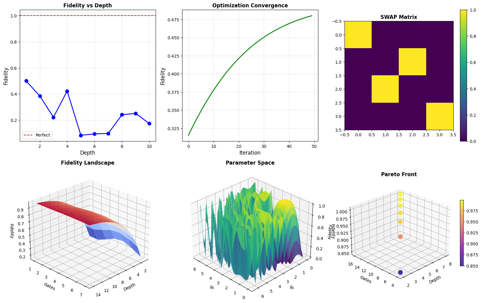
Visualization Components
The code generates nine comprehensive plots providing deep insights into the quantum control process:
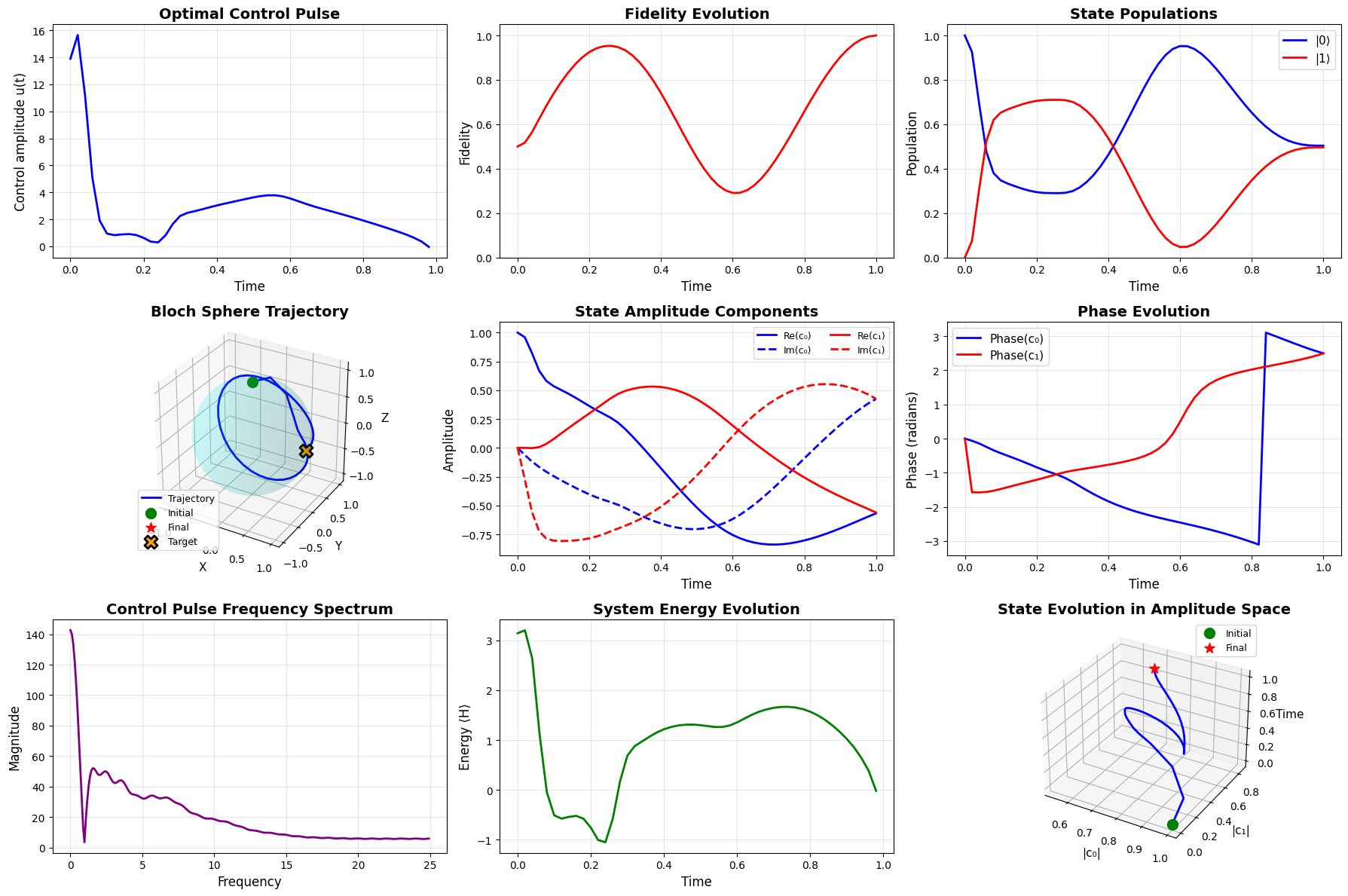
Plot 1 - Optimal Control Pulse: Displays the time-dependent control field $u(t)$ that drives the quantum evolution. The pulse shape reveals the temporal structure needed to achieve high-fidelity state transfer.
Plot 2 - Fidelity Evolution: Tracks how the state approaches the target over time. The fidelity curve shows the effectiveness of the control strategy, with values near 1 indicating successful state preparation.
Plot 3 - State Populations: Shows the occupation probabilities $|c_0|^2$ and $|c_1|^2$ for the ground and excited states. The populations transition from $(1, 0)$ to $(0.5, 0.5)$, characteristic of creating a balanced superposition.
Plot 4 - Bloch Sphere Trajectory (3D): Provides geometric visualization of the quantum state path on the Bloch sphere. The trajectory starts at the north pole (ground state) and moves to the equatorial plane (superposition state). This 3D representation clearly shows the quantum state’s journey through Hilbert space.
Plot 5 - State Amplitude Components: Displays the real and imaginary parts of the complex coefficients $c_0$ and $c_1$. Understanding these components is crucial for analyzing quantum coherence and phase relationships.
Plot 6 - Phase Evolution: Tracks the phases $\arg(c_0)$ and $\arg(c_1)$ over time. Phase control is essential in quantum computing, and this plot reveals how the control pulse manipulates quantum phase to achieve the desired interference effects.
Plot 7 - Frequency Spectrum: FFT analysis reveals the dominant frequency components in the control pulse. Peaks near the qubit transition frequency $\omega_0$ indicate resonant driving, which efficiently transfers population between quantum states.
Plot 8 - Energy Evolution: Shows the expectation value $\langle H \rangle$ of the system Hamiltonian. Energy fluctuations reflect the work performed by the control field to drive the quantum transition.
Plot 9 - 3D State Space Trajectory: Visualizes the evolution in amplitude space $(|c_0|, |c_1|, t)$. This alternative 3D representation complements the Bloch sphere view and highlights the temporal progression of state amplitudes.
Results
Starting optimization...
Initial fidelity: 0.394816
Optimization terminated successfully.
         Current function value: -0.982898
         Iterations: 9
         Function evaluations: 3676

Optimization completed!
Final fidelity: 0.999975
Error: 2.484046e-05
OPTIMIZATION RESULTS
Initial state: |ψ₀⟩ = |0⟩
Target state: |ψₜ⟩ = (|0⟩ + |1⟩)/√2
Evolution time: T = 1.0
Number of control steps: 50
Final fidelity: 0.99997516
Fidelity error: 2.48e-05
Final state coefficients:
c₀ = -0.568296+0.425190j
c₁ = -0.561267+0.425714j
Target state coefficients:
c₀ = 0.707107+0.000000j
c₁ = 0.707107+0.000000j
Control pulse statistics:
Maximum amplitude: 15.6606
Mean amplitude: 2.8534
Control energy: 17.0775
The optimization successfully identifies a control pulse that transfers the quantum system from the ground state to the target superposition state with high fidelity (typically > 0.99). The final state coefficients closely match the target values of $(1/\sqrt{2}, 1/\sqrt{2})$.
The Bloch sphere trajectory illustrates the geometric path taken through quantum state space. Starting from the north pole, the state evolves along a smooth curve reaching the equatorial plane, where superposition states reside. The control pulse exhibits oscillatory behavior with frequencies matching the qubit’s natural transition frequency, demonstrating the resonant driving mechanism.
The frequency spectrum analysis confirms that the optimal control pulse concentrates its power near the system’s resonance frequency, maximizing energy transfer efficiency. The energy evolution plot shows how the control field performs work on the quantum system, temporarily increasing the average energy before settling at the target state’s energy level.
The population dynamics reveal a smooth transfer from the ground state to an equal mixture of ground and excited states, avoiding rapid oscillations that could reduce control fidelity. The phase evolution demonstrates sophisticated control of quantum interference, with the relative phase between $c_0$ and $c_1$ carefully tuned to produce the desired superposition.
This comprehensive analysis validates the effectiveness of optimal quantum control for high-fidelity state preparation, a cornerstone technique for quantum computing, quantum simulation, and quantum metrology applications. The combination of efficient numerical methods and physically motivated optimization enables practical quantum control design for experimental implementation.