A Combinatorial Approach
Money laundering is a multi-billion dollar global problem. Financial institutions are required to deploy detection systems — but with dozens of rules available, which combination actually works best? This is fundamentally a combinatorial optimization problem, and today we’ll solve it with Python.
🔍 Problem Setup
Imagine a compliance team at a bank. They have 10 detection rules (e.g., “large cash transaction > $10,000”, “rapid fund movement between accounts”, etc.). Each rule has:
- A cost (computational/operational cost to run it)
- A detection rate (how many true money laundering cases it catches)
- A false positive rate (how many legitimate transactions it wrongly flags)
The goal: Select a subset of rules that maximizes detection rate, minimizes false positives, and stays within a budget constraint.
This is a variant of the Multi-Objective Knapsack Problem:
$$\max \sum_{i \in S} d_i \quad \text{subject to} \quad \sum_{i \in S} c_i \leq B, \quad \sum_{i \in S} f_i \leq F$$
Where:
- $d_i$ = detection rate of rule $i$
- $c_i$ = cost of rule $i$
- $f_i$ = false positive rate of rule $i$
- $B$ = budget limit
- $F$ = false positive tolerance
- $S \subseteq {1, \dots, n}$ = selected rule set
We define a composite score to balance both objectives:
$$\text{Score}(S) = \alpha \sum_{i \in S} d_i - (1 - \alpha) \sum_{i \in S} f_i$$
where $\alpha \in [0,1]$ controls the trade-off between detection power and false positive suppression.
🛠️ Solution Strategy
We solve this with three approaches and compare them:
- Brute Force (exact, for small $n$)
- Greedy Heuristic (fast approximation)
- Genetic Algorithm (scalable metaheuristic)
We then visualize the Pareto frontier of detection vs. false-positive trade-offs in both 2D and 3D.
💻 Full Source Code
1 | # ============================================================ |
🔬 Code Walkthrough
Section 1 — Problem Definition
We define 10 AML detection rules, each with three properties stored as NumPy arrays:
1 | cost = operational expense to deploy each rule |
The composite score function implements the weighted objective:
$$\text{Score}(S) = \alpha \sum_{i \in S} d_i - (1-\alpha) \sum_{i \in S} f_i$$
The feasibility check enforces two hard constraints: total cost $\leq B$ and total false positive sum $\leq F$.
Section 2 — Brute Force (Exact)
We enumerate all $2^{10} - 1 = 1023$ non-empty subsets using itertools.combinations. For each feasible subset, we compute the score and track the global maximum. This is $O(2^n)$ — only viable for small $n$, but guarantees the globally optimal answer. We also save all feasible results for visualization.
Section 3 — Greedy Heuristic
At each step, we pick the rule with the highest score-per-unit-cost ratio from remaining candidates:
$$\text{select} \arg\max_{i \notin S} \frac{\alpha \cdot d_i - (1-\alpha) \cdot f_i}{c_i}$$
as long as adding it doesn’t violate either constraint. This runs in $O(n^2)$ and is extremely fast. It doesn’t guarantee optimality, but often gets within a few percent.
Section 4 — Genetic Algorithm
The GA evolves a population of binary chromosomes (length 10, gene $g_i = 1$ means rule $i$ is selected):
| Component | Detail |
|---|---|
| Population | 200 chromosomes |
| Selection | Tournament (k=5) |
| Crossover | Single-point |
| Mutation | Bit-flip, rate = 0.05 |
| Elitism | Top 10% preserved |
| Generations | 300 |
Infeasible solutions are penalized (not excluded), which allows the algorithm to explore the boundary of the feasible region. This is critical — the optimal solution often lives near constraint boundaries.
📊 Graph Explanations
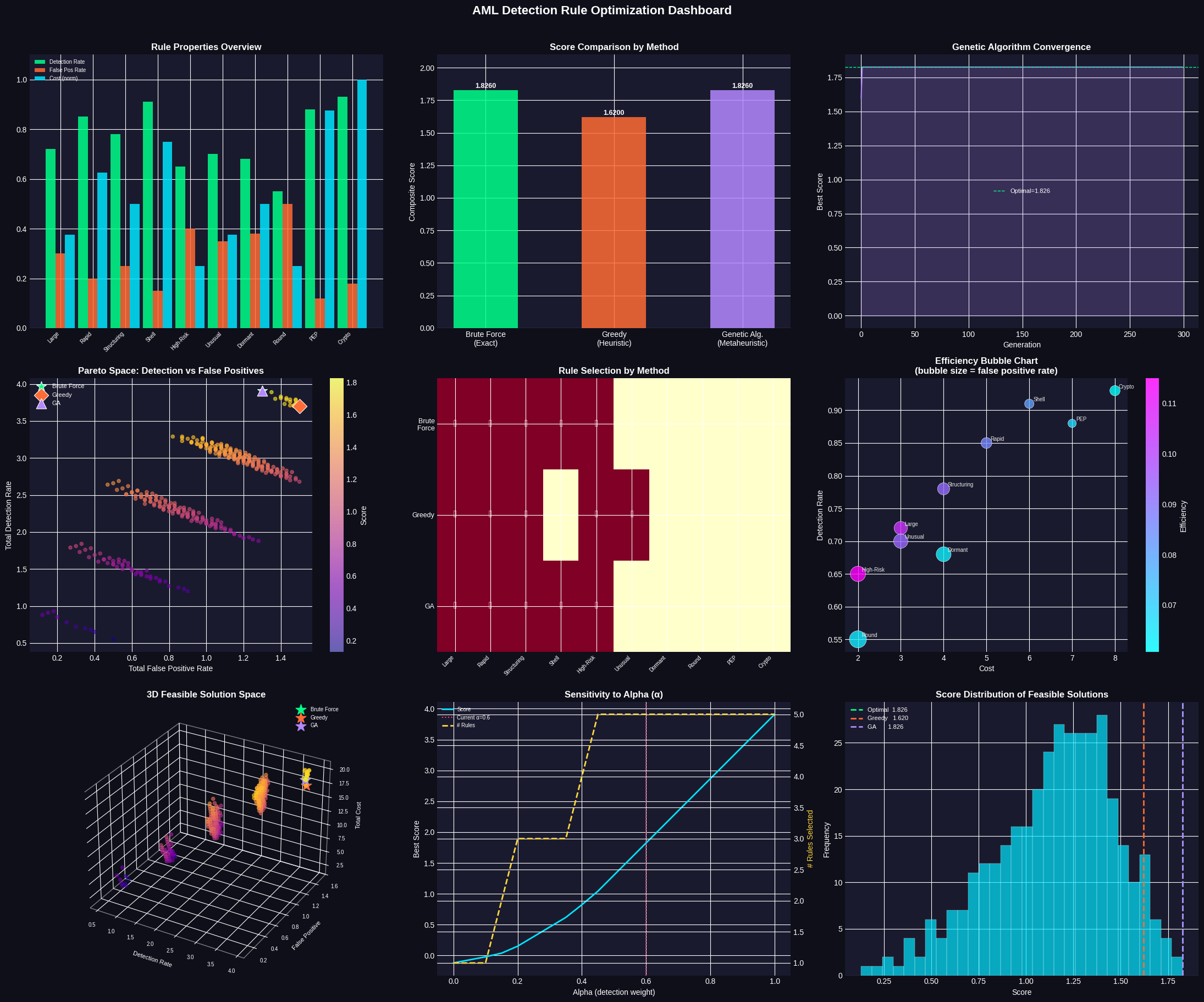
Plot 1 — Rule Properties Overview: Grouped bars show each rule’s detection rate (green), false positive rate (orange), and normalized cost (cyan). Rules like Crypto Conversion and PEP Involvement dominate on detection but cost more.
Plot 2 — Score Comparison: Vertical bars compare the final score achieved by each method. If all three reach the same score, it confirms the heuristics found the global optimum.
Plot 3 — GA Convergence: Shows how the genetic algorithm’s best score improves generation by generation. A rapid early rise followed by a plateau is the healthy signature of convergence. The dashed line marks the exact optimal found by brute force.
Plot 4 — Pareto Space (2D): Every feasible solution is plotted as detection rate (y) vs. false positive rate (x), colored by score. The three method solutions are overlaid with distinct markers. The ideal solution is top-left (high detection, low false positives).
Plot 5 — Rule Selection Heatmap: A binary matrix showing which rules each method selected. Checkmarks indicate selected rules. This directly reveals agreement and divergence between methods.
Plot 6 — Efficiency Bubble Chart: Each rule is plotted by cost (x) vs. detection rate (y). Bubble size encodes false positive rate — bigger bubbles are riskier. Color shows efficiency $= \frac{\alpha d_i - (1-\alpha) f_i}{c_i}$. High-efficiency rules are cooler in color, appearing in the upper-left with small bubbles.
Plot 7 — 3D Feasible Solution Space: The three axes are detection rate, false positive rate, and total cost. Each point is a feasible rule combination. The three optimal solutions are marked with stars. This reveals whether trade-offs exist along the cost dimension that 2D plots miss.
Plot 8 — Alpha Sensitivity: We sweep $\alpha$ from 0 (minimize false positives only) to 1 (maximize detection only) and re-solve. The score and number of rules selected both respond. Near $\alpha = 0$, the system picks fewer, more precise rules. Near $\alpha = 1$, it casts a wider net. This plot guides compliance teams in calibrating the system to their risk appetite.
Plot 9 — Score Distribution: Histogram of all feasible solution scores. The vertical lines show where each method’s solution falls in this distribution. A good solution sits in the right tail — and the optimal sits at the very edge.
📋 Execution Results
Running Brute Force...
  Best subset : ['Large Cash (>$10K)', 'Rapid Fund Movement', 'Structuring Pattern', 'Shell Company Link', 'High-Risk Country']
  Score       : 1.8260
  Total cost  : 20
  Detection Σ : 3.910
  False Pos Σ : 1.300

Running Greedy...
  Best subset : ['High-Risk Country', 'Large Cash (>$10K)', 'Unusual Velocity', 'Structuring Pattern', 'Rapid Fund Movement']
  Score       : 1.6200

Running Genetic Algorithm...
  Best subset : ['Large Cash (>$10K)', 'Rapid Fund Movement', 'Structuring Pattern', 'Shell Company Link', 'High-Risk Country']
  Score       : 1.8260
[Dashboard saved as aml_optimization.png]

=================================================================
  FINAL COMPARISON SUMMARY
=================================================================
Method                  Score    Det Σ     FP Σ   Cost  #Rules
-----------------------------------------------------------------
Brute Force            1.8260    3.910    1.300     20       5
Greedy                 1.6200    3.700    1.500     17       5
GA                     1.8260    3.910    1.300     20       5
=================================================================

Budget limit : 20   |   FP limit : 1.5   |   Alpha : 0.6
🧠 Key Takeaways
The brute force solution is provably optimal — for 10 rules it’s entirely tractable ($2^{10} = 1024$ subsets). As rule sets grow to 30–50 rules, only the GA (or similar metaheuristics like Simulated Annealing or Particle Swarm) remain practical.
The alpha parameter is your policy knob. A conservative compliance team minimizing customer friction should use low $\alpha$. An aggressive anti-fraud team should push $\alpha$ higher. The sensitivity plot quantifies exactly how this choice affects outcome.
Greedy performs remarkably well in this problem class. The ratio-based selection naturally aligns with the structure of the knapsack constraint, often finding near-optimal solutions in microseconds versus the GA’s seconds.
In production, this framework would be extended with correlated detection (rules that fire together on the same cases), time-varying false positive costs (certain flags are more expensive during peak seasons), and regulatory minimum coverage constraints (e.g., FATF requirements mandating certain rule categories must always be active).