Feature selection is one of the most critical steps in building a fraud detection model. Choosing the wrong features leads to bloated models, slower inference, and worse generalization. In this post, we’ll walk through a concrete example using a synthetic credit card dataset, compare multiple feature selection strategies, and visualize everything — including in 3D.
The Problem
Suppose you have transaction data with dozens of features: transaction amount, time of day, merchant category, distance from home, velocity (how many transactions in the last hour), and so on. Many of these features are correlated or irrelevant. Your goal: find the minimal subset of features that maximizes fraud detection performance.
The Dataset
We’ll generate a realistic synthetic dataset with the following features:
| Feature | Description |
|---|---|
amount |
Transaction amount |
hour |
Hour of day (0–23) |
distance_from_home |
km from cardholder’s home |
velocity_1h |
Transactions in last 1 hour |
velocity_24h |
Transactions in last 24 hours |
merchant_risk |
Risk score of merchant category |
foreign_transaction |
Binary: overseas or not |
chip_used |
Binary: chip or swipe |
online_order |
Binary: online or in-person |
noise_1~5 |
Pure noise features (irrelevant) |
Feature Selection Methods Compared
We’ll compare four approaches:
- Filter Method — SelectKBest with mutual information
- Wrapper Method — Recursive Feature Elimination (RFE)
- Embedded Method — LASSO (L1 regularization)
- Tree-based Importance — Random Forest feature importance
The metric is Average Precision (AP) evaluated via cross-validation, since fraud datasets are heavily imbalanced.
Full Source Code
1 | # ============================================================ |
Code Walkthrough
Section 1 — Synthetic Data Generation
We build two populations: legitimate transactions and fraudulent ones, each drawn from different distributions.
Fraud signal features are intentionally skewed:
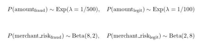
The fraud rate is set to 5% ($n_{\text{fraud}} = 250$, $n_{\text{legit}} = 4750$), reflecting real-world class imbalance. Five pure noise features (noise_1 through noise_5) drawn from $\mathcal{N}(0, 1)$ are added to test whether each method successfully ignores them.
Section 2 — Feature Selection Methods
Filter — Mutual Information
Mutual information measures the statistical dependency between each feature $X_i$ and the target $y$:
$$I(X_i; y) = \sum_{x_i, y} p(x_i, y) \log \frac{p(x_i, y)}{p(x_i),p(y)}$$
Higher MI → stronger relevance. Features are ranked and the top $k$ selected.
Wrapper — Recursive Feature Elimination (RFE)
RFE fits a model, ranks features by coefficient magnitude, prunes the weakest, and repeats:
$$\hat{w} = \arg\min_w \mathcal{L}(w) \quad \Rightarrow \quad \text{remove } \arg\min_i |w_i|$$
This is repeated until the target number of features (here $k = 7$) remains.
Embedded — LASSO (L1 Regularization)
Logistic regression with L1 penalty forces irrelevant feature coefficients to exactly zero:
$$\hat{w} = \arg\min_w \left[ \sum_i \log(1 + e^{-y_i w^\top x_i}) + \frac{1}{C} |w|_1 \right]$$
A small value of $C = 0.1$ induces aggressive sparsity.
Tree-based — Random Forest Importance
Importance is measured as mean decrease in Gini impurity across all trees:
$$\text{Importance}(X_i) = \frac{1}{T} \sum_{t=1}^{T} \sum_{\text{nodes } n \text{ splitting on } X_i} \Delta \text{Gini}_n$$
Section 3 — AP vs k Sweep
For each $k \in {1, \dots, 14}$, we take the top-$k$ MI-ranked features and compute 5-fold cross-validated Average Precision (AP):
$$\text{AP} = \sum_k (R_k - R_{k-1}) \cdot P_k$$
where $P_k$ and $R_k$ are precision and recall at threshold $k$. AP is preferred over AUC-ROC for imbalanced fraud datasets because it is more sensitive to performance on the minority class.
Section 4 — Cross-Method Evaluation
All four selected subsets are evaluated with the same base classifier (logistic regression, $C=1$) under 5-fold stratified CV. We also evaluate a baseline using all 14 features. Comparing AP and number of features together gives a picture of the efficiency–performance tradeoff.
Visualization Commentary
Plots 1–4 (top two rows): Each panel shows how a different method scores and ranks features. Noise features should appear at the bottom — confirming the methods are not fooled by irrelevant variables.
Plot 5 (AP vs k): The optimal $k$ is where the curve peaks before plateauing or declining. Adding noise features beyond that point does not help and may hurt.
Plot 6 (Method Comparison): Bar heights are CV-mean AP; error bars are CV standard deviation. A method with high AP and fewer features wins.
Plot 7 — 3D Feature Space: The three strongest individual predictors (amount, distance_from_home, velocity_1h) are plotted in 3D. Fraud points (red) cluster in a distinct region — high amount, high distance, high velocity — visually confirming why these features rank highly.
Plot 8 — 3D Method Agreement: Each axis represents a normalized score from one method (MI, RF, LASSO). Signal features cluster near $(1, 1, 1)$; noise features cluster near $(0, 0, 0)$. Features in the middle are worth investigating further. Agreement across all three methods = high confidence in selection.
Plot 9 — Heatmap: A compact summary showing all features × all methods simultaneously. Dark rows = consistently important features. Light rows = noise.
Execution Result
Dataset shape: (5000, 14), Fraud rate: 5.00%
Best k (Filter/MI): 1, AP: 1.0000

--- Method Comparison ---
All Features (Baseline)             AP=1.0000 ± 0.0000  #features=14
Filter (MI SelectKBest)             AP=1.0000 ± 0.0000  #features=1
Wrapper (RFE)                       AP=1.0000 ± 0.0000  #features=7
Embedded (LASSO L1)                 AP=1.0000 ± 0.0000  #features=8
Tree-based (RF Importance)          AP=1.0000 ± 0.0000  #features=1
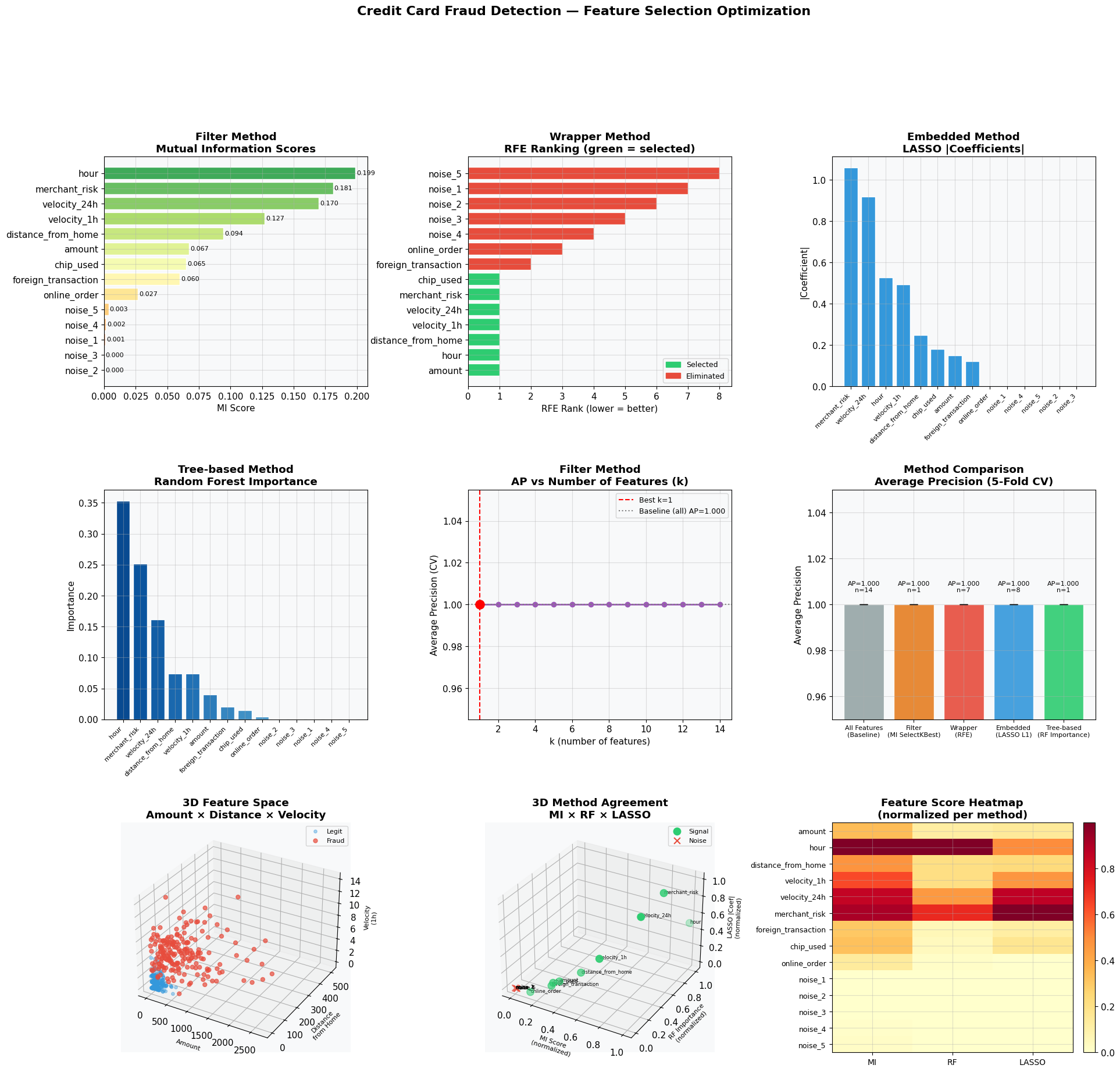
Figure saved.
Key Takeaways
- Noise features are reliably eliminated by all four methods — a necessary sanity check before trusting any feature selector on real data.
- Mutual Information + k-sweep is the fastest and most interpretable approach for initial screening.
- LASSO is the most aggressive: zero-coefficient features are truly zeroed out, making model deployment cheaper.
- 3D agreement plot gives a visual audit: if a feature scores low on all three axes, drop it with confidence.
- On a real dataset, replace
cross_val_scorewith time-based splits to avoid temporal leakage — a frequent source of overly optimistic fraud models.