Optimizing Real-Time Monitoring Alert Thresholds to Minimize Operational Load

Real-time monitoring systems are essential in modern infrastructure, but poorly tuned alert thresholds lead to alert fatigue — operators become overwhelmed by false positives and start ignoring alerts entirely. The goal is to find the sweet spot: catch real incidents without drowning the team in noise.

In this post, we’ll build a complete optimization pipeline from scratch using a concrete example: a web server CPU monitoring system.


Problem Setup

Imagine you have a fleet of web servers. Your monitoring system checks CPU usage every minute and fires an alert when usage exceeds a threshold $\theta$. The challenge:

  • If $\theta$ is too low → too many false alerts → operator fatigue
  • If $\theta$ is too high → real incidents get missed → downtime

We want to find $\theta^*$ that minimizes a cost function balancing false positives and missed detections.


The Math

Let $X \sim \mathcal{N}(\mu, \sigma^2)$ be the CPU usage distribution under normal operation, and let $X_{inc} \sim \mathcal{N}(\mu_{inc}, \sigma_{inc}^2)$ be the distribution during an incident.

False Positive Rate:

$$FPR(\theta) = P(X > \theta) = 1 - \Phi\left(\frac{\theta - \mu}{\sigma}\right)$$

False Negative Rate (Miss Rate):

$$FNR(\theta) = P(X_{inc} \leq \theta) = \Phi\left(\frac{\theta - \mu_{inc}}{\sigma_{inc}}\right)$$

Total Operational Cost:

$$C(\theta) = \lambda_{fp} \cdot FPR(\theta) + \lambda_{fn} \cdot FNR(\theta) + \lambda_{vol} \cdot \overline{V}(\theta)$$

where:

  • $\lambda_{fp}$ = cost weight for false positives (operator time wasted)
  • $\lambda_{fn}$ = cost weight for missed incidents (business impact)
  • $\lambda_{vol}$ = cost weight for alert volume
  • $\overline{V}(\theta)$ = expected alert volume per hour

Optimal threshold:

$$\theta^* = \arg\min_{\theta} , C(\theta)$$


Concrete Example

Parameter Value
Normal CPU mean $\mu$ 45%
Normal CPU std $\sigma$ 10%
Incident CPU mean $\mu_{inc}$ 80%
Incident CPU std $\sigma_{inc}$ 8%
Incident frequency 5 per day
$\lambda_{fp}$ 1.0
$\lambda_{fn}$ 10.0
$\lambda_{vol}$ 0.5

Full Python Implementation

1
2
3
4
5
6
7
8
9
10
11
12
13
14
15
16
17
18
19
20
21
22
23
24
25
26
27
28
29
30
31
32
33
34
35
36
37
38
39
40
41
42
43
44
45
46
47
48
49
50
51
52
53
54
55
56
57
58
59
60
61
62
63
64
65
66
67
68
69
70
71
72
73
74
75
76
77
78
79
80
81
82
83
84
85
86
87
88
89
90
91
92
93
94
95
96
97
98
99
100
101
102
103
104
105
106
107
108
109
110
111
112
113
114
115
116
117
118
119
120
121
122
123
124
125
126
127
128
129
130
131
132
133
134
135
136
137
138
139
140
141
142
143
144
145
146
147
148
149
150
151
152
153
154
155
156
157
158
159
160
161
162
163
164
165
166
167
168
169
170
171
172
173
174
175
176
177
178
179
180
181
182
183
184
185
186
187
188
189
190
191
192
193
194
195
196
197
198
199
200
201
202
203
204
205
206
207
208
209
210
211
212
213
214
215
216
217
218
219
220
221
222
223
224
225
226
227
228
229
230
231
232
233
234
235
236
237
238
239
240
241
242
243
244
245
246
247
248
249
250
251
252
253
254
255
256
257
258
259
260
261
262
263
264
265
266
267
268
269
270
271
272
273
274
275
276
277
278
279
280
281
282
283
284
285
286
287
288
289
290
291
292
293
294
295
296
297
298
299
300
301
302
303
304
305
306
307
308
309
310
311
312
313
314
315
316
317
318
319
320
321
322
323
324
325
326
327
328
329
330
331
332
333
334
335
336
337
338
339
340
341
342
343
344
345
346
347
348
349
350
351
352
353
354
355
356
357
358
359
360
361
362
363
364
365
366
367
# ============================================================
# Real-Time Monitoring Alert Threshold Optimization
# Minimizing Operational Load
# ============================================================

import numpy as np
import matplotlib.pyplot as plt
import matplotlib.patches as mpatches
from matplotlib import cm
from scipy import stats
from scipy.optimize import minimize_scalar, minimize
from scipy.stats import norm
from mpl_toolkits.mplot3d import Axes3D
import warnings
warnings.filterwarnings('ignore')

# ── Seaborn-style without importing seaborn ──────────────────
plt.rcParams.update({
'axes.facecolor': '#f8f9fa',
'figure.facecolor': 'white',
'axes.grid': True,
'grid.color': 'white',
'grid.linewidth': 1.2,
'axes.spines.top': False,
'axes.spines.right': False,
'font.size': 11,
})

# ============================================================
# 1. System Parameters
# ============================================================
# Normal operation distribution
MU_NORMAL = 45.0 # mean CPU % under normal load
SIGMA_NORMAL = 10.0 # std CPU % under normal load

# Incident distribution
MU_INC = 80.0 # mean CPU % during incident
SIGMA_INC = 8.0 # std CPU % during incident

# Cost weights
LAMBDA_FP = 1.0 # false-positive cost (wasted operator time)
LAMBDA_FN = 10.0 # false-negative cost (missed incident / business impact)
LAMBDA_VOL = 0.5 # alert-volume cost (noise fatigue)

# Operational context
INCIDENTS_PER_DAY = 5
CHECKS_PER_HOUR = 60
HOURS_PER_DAY = 24
CHECKS_PER_DAY = CHECKS_PER_HOUR * HOURS_PER_DAY

# ============================================================
# 2. Core Functions (vectorised for speed)
# ============================================================
def fpr(theta, mu=MU_NORMAL, sigma=SIGMA_NORMAL):
"""False Positive Rate: P(X > theta | normal)"""
return 1.0 - norm.cdf(theta, loc=mu, scale=sigma)

def fnr(theta, mu=MU_INC, sigma=SIGMA_INC):
"""False Negative Rate: P(X <= theta | incident)"""
return norm.cdf(theta, loc=mu, scale=sigma)

def alert_volume_per_hour(theta):
"""Expected number of alerts fired per hour."""
# Normal alerts (false positives)
normal_checks = CHECKS_PER_HOUR
vol_normal = normal_checks * fpr(theta)

# Incident alerts (true positives) — incident lasts ~15 min on average
incident_checks_per_hour = (INCIDENTS_PER_DAY / HOURS_PER_DAY) * 15
vol_incident = incident_checks_per_hour * (1.0 - fnr(theta))

return vol_normal + vol_incident

def operational_cost(theta):
"""
Total cost C(theta) = lambda_fp * FPR + lambda_fn * FNR + lambda_vol * V_bar
Vectorised: theta can be a scalar or ndarray.
"""
theta = np.asarray(theta, dtype=float)
fp = fpr(theta)
fn = fnr(theta)
vol = alert_volume_per_hour(theta)
# Normalise volume to [0,1] range for comparability
vol_norm = vol / CHECKS_PER_HOUR
return LAMBDA_FP * fp + LAMBDA_FN * fn + LAMBDA_VOL * vol_norm

# ============================================================
# 3. Optimisation (scipy.optimize — fast bounded search)
# ============================================================
result = minimize_scalar(
operational_cost,
bounds=(MU_NORMAL, MU_INC),
method='bounded',
options={'xatol': 1e-6}
)
THETA_OPT = result.x
COST_OPT = result.fun

# Sensitivity: how cost changes ±5 pp around optimum
DELTA = 5.0
cost_low = operational_cost(THETA_OPT - DELTA)
cost_high = operational_cost(THETA_OPT + DELTA)

print("=" * 55)
print(" ALERT THRESHOLD OPTIMISATION RESULTS")
print("=" * 55)
print(f" Optimal threshold θ* : {THETA_OPT:.2f}%")
print(f" Minimum cost C* : {COST_OPT:.4f}")
print(f" FPR at θ* : {fpr(THETA_OPT)*100:.2f}%")
print(f" FNR at θ* : {fnr(THETA_OPT)*100:.2f}%")
print(f" Alert volume/hr V̄ : {alert_volume_per_hour(THETA_OPT):.2f} alerts")
print(f" Cost at θ*-5pp : {cost_low:.4f} (Δ={cost_low-COST_OPT:+.4f})")
print(f" Cost at θ*+5pp : {cost_high:.4f} (Δ={cost_high-COST_OPT:+.4f})")
print("=" * 55)

# ============================================================
# 4. Multi-weight Sensitivity Grid (vectorised, fast)
# ============================================================
lam_fp_vals = np.linspace(0.5, 5.0, 40)
lam_fn_vals = np.linspace(1.0, 20.0, 40)
LFP, LFN = np.meshgrid(lam_fp_vals, lam_fn_vals)

# For each (lam_fp, lam_fn) combo, find optimal theta via a dense grid search
# (faster than calling minimize_scalar 1600 times)
theta_grid = np.linspace(MU_NORMAL, MU_INC, 500)
fp_grid = fpr(theta_grid)
fn_grid = fnr(theta_grid)
vol_grid = alert_volume_per_hour(theta_grid) / CHECKS_PER_HOUR

# Shape: (len_lam_fp, len_lam_fn, len_theta)
cost_3d = (
LFP[:, :, np.newaxis] * fp_grid[np.newaxis, np.newaxis, :]
+ LFN[:, :, np.newaxis] * fn_grid[np.newaxis, np.newaxis, :]
+ LAMBDA_VOL * vol_grid[np.newaxis, np.newaxis, :]
)
opt_idx = np.argmin(cost_3d, axis=2)
THETA_SURF = theta_grid[opt_idx] # (40, 40) surface

# ============================================================
# 5. Simulate a 24-hour time series
# ============================================================
rng = np.random.default_rng(42)
t = np.arange(0, CHECKS_PER_DAY)

# Base CPU: sinusoidal daily cycle + noise
cpu_base = (
MU_NORMAL
+ 8.0 * np.sin(2 * np.pi * t / CHECKS_PER_DAY)
+ rng.normal(0, SIGMA_NORMAL * 0.7, size=len(t))
)

# Inject 5 incidents
incident_times = rng.choice(t[200:-200], size=INCIDENTS_PER_DAY, replace=False)
cpu_sim = cpu_base.copy()
for it in incident_times:
dur = rng.integers(10, 40)
end = min(it + dur, CHECKS_PER_DAY)
cpu_sim[it:end] += rng.normal(MU_INC - MU_NORMAL, SIGMA_INC * 0.5, size=end - it)

# Alert flags for multiple thresholds
THETA_NAIVE = 70.0 # typical naive threshold
alerts_opt = cpu_sim > THETA_OPT
alerts_naive = cpu_sim > THETA_NAIVE

# ============================================================
# 6. Plots
# ============================================================
fig = plt.figure(figsize=(22, 26))
fig.suptitle(
"Real-Time Monitoring Alert Threshold Optimisation\n"
"Minimising Operational Load",
fontsize=16, fontweight='bold', y=0.98
)

COLOR_OPT = '#2ecc71'
COLOR_NAIVE = '#e74c3c'
COLOR_FPR = '#3498db'
COLOR_FNR = '#e67e22'
COLOR_COST = '#9b59b6'

theta_range = np.linspace(20, 100, 800)

# ── Plot 1: CPU distributions ─────────────────────────────
ax1 = fig.add_subplot(4, 2, 1)
x = np.linspace(0, 120, 1000)
ax1.fill_between(x, norm.pdf(x, MU_NORMAL, SIGMA_NORMAL),
alpha=0.35, color=COLOR_FPR, label='Normal operation')
ax1.fill_between(x, norm.pdf(x, MU_INC, SIGMA_INC),
alpha=0.35, color=COLOR_NAIVE, label='Incident')
ax1.plot(x, norm.pdf(x, MU_NORMAL, SIGMA_NORMAL), color=COLOR_FPR, lw=2)
ax1.plot(x, norm.pdf(x, MU_INC, SIGMA_INC), color=COLOR_NAIVE, lw=2)
ax1.axvline(THETA_OPT, color=COLOR_OPT, lw=2.5, ls='--', label=f'θ* = {THETA_OPT:.1f}%')
ax1.axvline(THETA_NAIVE, color=COLOR_NAIVE, lw=2, ls=':', label=f'θ_naive = {THETA_NAIVE}%')
ax1.set_xlabel('CPU Usage (%)'); ax1.set_ylabel('Density')
ax1.set_title('CPU Distribution: Normal vs Incident')
ax1.legend(fontsize=9)

# ── Plot 2: FPR & FNR curves ──────────────────────────────
ax2 = fig.add_subplot(4, 2, 2)
ax2.plot(theta_range, fpr(theta_range) * 100, color=COLOR_FPR, lw=2.5, label='FPR (%)')
ax2.plot(theta_range, fnr(theta_range) * 100, color=COLOR_FNR, lw=2.5, label='FNR (%)')
ax2.axvline(THETA_OPT, color=COLOR_OPT, lw=2.5, ls='--', label=f'θ* = {THETA_OPT:.1f}%')
ax2.axvline(THETA_NAIVE, color=COLOR_NAIVE, lw=2, ls=':', label=f'θ_naive = {THETA_NAIVE}%')
ax2.set_xlabel('Threshold θ (%)'); ax2.set_ylabel('Rate (%)')
ax2.set_title('False Positive / Negative Rates vs Threshold')
ax2.legend(fontsize=9)

# ── Plot 3: Cost function ─────────────────────────────────
ax3 = fig.add_subplot(4, 2, 3)
cost_vals = operational_cost(theta_range)
ax3.plot(theta_range, cost_vals, color=COLOR_COST, lw=2.5)
ax3.axvline(THETA_OPT, color=COLOR_OPT, lw=2.5, ls='--', label=f'θ* = {THETA_OPT:.1f}%')
ax3.axvline(THETA_NAIVE, color=COLOR_NAIVE, lw=2, ls=':', label=f'θ_naive = {THETA_NAIVE}%')
ax3.scatter([THETA_OPT], [COST_OPT], color=COLOR_OPT, s=120, zorder=5)
ax3.set_xlabel('Threshold θ (%)'); ax3.set_ylabel('Cost C(θ)')
ax3.set_title('Operational Cost vs Threshold')
ax3.legend(fontsize=9)

# ── Plot 4: Alert volume ───────────────────────────────────
ax4 = fig.add_subplot(4, 2, 4)
vol_vals = alert_volume_per_hour(theta_range)
ax4.plot(theta_range, vol_vals, color='#1abc9c', lw=2.5)
ax4.axvline(THETA_OPT, color=COLOR_OPT, lw=2.5, ls='--', label=f'θ* = {THETA_OPT:.1f}%')
ax4.axvline(THETA_NAIVE, color=COLOR_NAIVE, lw=2, ls=':', label=f'θ_naive = {THETA_NAIVE}%')
ax4.set_xlabel('Threshold θ (%)'); ax4.set_ylabel('Alerts / Hour')
ax4.set_title('Expected Alert Volume per Hour')
ax4.legend(fontsize=9)

# ── Plot 5 & 6: 24-hour simulation ────────────────────────
hours = t / CHECKS_PER_HOUR
ax5 = fig.add_subplot(4, 2, (5, 6))
ax5.plot(hours, cpu_sim, color='#95a5a6', lw=0.8, alpha=0.7, label='CPU usage')
ax5.axhline(THETA_OPT, color=COLOR_OPT, lw=2, ls='--', label=f'θ* = {THETA_OPT:.1f}%')
ax5.axhline(THETA_NAIVE, color=COLOR_NAIVE, lw=2, ls=':', label=f'θ_naive = {THETA_NAIVE}%')
# Shade alerts
ax5.fill_between(hours, cpu_sim, THETA_OPT,
where=alerts_opt, alpha=0.4, color=COLOR_OPT, label='Alert (opt)')
ax5.fill_between(hours, cpu_sim, THETA_NAIVE,
where=alerts_naive, alpha=0.25, color=COLOR_NAIVE, label='Alert (naive)')
# Mark incidents
for it in incident_times:
ax5.axvline(it / CHECKS_PER_HOUR, color='black', lw=1, ls=':', alpha=0.5)
ax5.set_xlabel('Time (hours)'); ax5.set_ylabel('CPU Usage (%)')
ax5.set_title('Simulated 24-Hour CPU Timeline with Alerts')
ax5.legend(fontsize=9, ncol=3)

# ── Plot 7: ROC-style trade-off ───────────────────────────
ax6 = fig.add_subplot(4, 2, 7)
fpr_vals = fpr(theta_range) * 100
fnr_vals = fnr(theta_range) * 100
sc = ax6.scatter(fpr_vals, fnr_vals,
c=theta_range, cmap='plasma', s=8, zorder=3)
plt.colorbar(sc, ax=ax6, label='Threshold θ (%)')
ax6.scatter([fpr(THETA_OPT) * 100], [fnr(THETA_OPT) * 100],
color=COLOR_OPT, s=200, zorder=5, marker='*', label='θ*')
ax6.scatter([fpr(THETA_NAIVE) * 100], [fnr(THETA_NAIVE) * 100],
color=COLOR_NAIVE, s=150, zorder=5, marker='D', label='θ_naive')
ax6.set_xlabel('FPR (%)'); ax6.set_ylabel('FNR (%)')
ax6.set_title('FPR vs FNR Trade-Off Curve')
ax6.legend(fontsize=9)

# ── Plot 8: Cost decomposition bar ───────────────────────
ax7 = fig.add_subplot(4, 2, 8)
thetas_bar = [THETA_OPT, THETA_NAIVE, 60.0, 55.0]
labels_bar = [f'θ*={THETA_OPT:.1f}%', 'Naive=70%', 'θ=60%', 'θ=55%']
c_fp = [LAMBDA_FP * fpr(th) for th in thetas_bar]
c_fn = [LAMBDA_FN * fnr(th) for th in thetas_bar]
c_vol = [LAMBDA_VOL * alert_volume_per_hour(th) / CHECKS_PER_HOUR for th in thetas_bar]
x_pos = np.arange(len(thetas_bar))
w = 0.55
ax7.bar(x_pos, c_fp, w, label='FP cost', color=COLOR_FPR, alpha=0.85)
ax7.bar(x_pos, c_fn, w, bottom=c_fp,
label='FN cost', color=COLOR_FNR, alpha=0.85)
ax7.bar(x_pos, c_vol, w,
bottom=np.array(c_fp) + np.array(c_fn),
label='Volume cost', color='#95a5a6', alpha=0.85)
ax7.set_xticks(x_pos); ax7.set_xticklabels(labels_bar, fontsize=10)
ax7.set_ylabel('Cost'); ax7.set_title('Cost Decomposition by Threshold')
ax7.legend(fontsize=9)

plt.tight_layout(rect=[0, 0, 1, 0.97])
plt.savefig('alert_opt_2d.png', dpi=150, bbox_inches='tight')
plt.show()
print("[Figure 1 — 2D dashboard saved]")

# ============================================================
# 7. 3D Surface: Optimal Threshold over (λ_fp, λ_fn) space
# ============================================================
fig2 = plt.figure(figsize=(20, 14))
fig2.suptitle('3D Sensitivity Analysis: Optimal Threshold Surface',
fontsize=15, fontweight='bold')

# ── 3D surface ────────────────────────────────────────────
ax3d = fig2.add_subplot(2, 2, (1, 2), projection='3d')
surf = ax3d.plot_surface(
LFP, LFN, THETA_SURF,
cmap='viridis', alpha=0.88, edgecolor='none'
)
ax3d.set_xlabel('λ_fp (FP weight)', labelpad=10)
ax3d.set_ylabel('λ_fn (FN weight)', labelpad=10)
ax3d.set_zlabel('Optimal θ* (%)', labelpad=10)
ax3d.set_title('Optimal Threshold θ* as a Function of Cost Weights')
fig2.colorbar(surf, ax=ax3d, shrink=0.5, label='θ* (%)')

# Mark current weights on surface
idx_fp = np.argmin(np.abs(lam_fp_vals - LAMBDA_FP))
idx_fn = np.argmin(np.abs(lam_fn_vals - LAMBDA_FN))
ax3d.scatter(
[LAMBDA_FP], [LAMBDA_FN], [THETA_SURF[idx_fn, idx_fp]],
color='red', s=150, zorder=10, label='Current weights'
)
ax3d.legend()

# ── 3D cost landscape for fixed weights ───────────────────
ax3d2 = fig2.add_subplot(2, 2, 3, projection='3d')
theta_g = np.linspace(40, 95, 120)
lam_fn_g = np.linspace(1, 20, 120)
TH, LN = np.meshgrid(theta_g, lam_fn_g)
COST_LAND = (
LAMBDA_FP * fpr(TH)
+ LN * fnr(TH)
+ LAMBDA_VOL * alert_volume_per_hour(TH) / CHECKS_PER_HOUR
)
surf2 = ax3d2.plot_surface(TH, LN, COST_LAND, cmap='inferno', alpha=0.85, edgecolor='none')
ax3d2.set_xlabel('Threshold θ (%)', labelpad=8)
ax3d2.set_ylabel('λ_fn', labelpad=8)
ax3d2.set_zlabel('Cost C(θ)', labelpad=8)
ax3d2.set_title('Cost Landscape: θ vs λ_fn')
fig2.colorbar(surf2, ax=ax3d2, shrink=0.5, label='Cost')

# ── Heatmap of optimal threshold ──────────────────────────
ax_hm = fig2.add_subplot(2, 2, 4)
hm = ax_hm.contourf(LFP, LFN, THETA_SURF, levels=25, cmap='viridis')
fig2.colorbar(hm, ax=ax_hm, label='θ* (%)')
ax_hm.contour(LFP, LFN, THETA_SURF, levels=10, colors='white', linewidths=0.6, alpha=0.5)
ax_hm.scatter([LAMBDA_FP], [LAMBDA_FN], color='red', s=180,
marker='*', label='Current', zorder=5)
ax_hm.set_xlabel('λ_fp'); ax_hm.set_ylabel('λ_fn')
ax_hm.set_title('Optimal Threshold Heatmap (λ_fp × λ_fn)')
ax_hm.legend()

plt.tight_layout()
plt.savefig('alert_opt_3d.png', dpi=150, bbox_inches='tight')
plt.show()
print("[Figure 2 — 3D sensitivity surface saved]")

# ============================================================
# 8. Summary statistics table
# ============================================================
print("\n" + "=" * 60)
print(" COMPARATIVE PERFORMANCE TABLE")
print("=" * 60)
print(f"{'Metric':<30} {'θ*='+str(round(THETA_OPT,1))+'%':>12} {'θ=70%':>10} {'θ=60%':>10}")
print("-" * 60)
for th, label in [(THETA_OPT, f'θ*={THETA_OPT:.1f}%'), (70.0, 'θ=70%'), (60.0, 'θ=60%')]:
pass # just for reference — table built below

rows = [
('FPR (%)', lambda t: f'{fpr(t)*100:.2f}%'),
('FNR (%)', lambda t: f'{fnr(t)*100:.2f}%'),
('Alerts/hr', lambda t: f'{alert_volume_per_hour(t):.2f}'),
('Total cost C(θ)', lambda t: f'{operational_cost(t):.4f}'),
]
for name, fn in rows:
vals = [fn(t) for t in [THETA_OPT, 70.0, 60.0]]
print(f'{name:<30} {vals[0]:>12} {vals[1]:>10} {vals[2]:>10}')
print("=" * 60)

Code Walkthrough

Section 1 – Parameters

We define two Gaussian distributions: one for normal CPU behavior ($\mu=45%$, $\sigma=10%$) and one for incident behavior ($\mu_{inc}=80%$, $\sigma_{inc}=8%$). Cost weights reflect real business priorities: a missed incident ($\lambda_{fn}=10$) costs 10× more than a false alarm.

Section 2 – Core Functions

fpr(theta) and fnr(theta) use scipy.stats.norm.cdf — these are vectorised over NumPy arrays, so we can evaluate thousands of thresholds in microseconds. alert_volume_per_hour(theta) estimates total alerts fired, combining both normal-operation false positives and incident true positives (assuming a 15-minute average incident duration).

Section 3 – Optimisation

We use scipy.optimize.minimize_scalar with method='bounded', which applies Brent’s method — a derivative-free algorithm that achieves superlinear convergence. The bounded search over $[\mu, \mu_{inc}]$ avoids trivially bad solutions. This is far faster than a brute-force grid search.

Why not gradient descent? The cost function $C(\theta)$ is smooth and unimodal in this range, making bounded scalar optimisation ideal. For multi-dimensional threshold problems (multiple metrics), you’d switch to scipy.optimize.minimize with L-BFGS-B.

Section 4 – Sensitivity Grid

Instead of calling minimize_scalar 1,600 times (once per $(\lambda_{fp}, \lambda_{fn})$ pair), we pre-compute FPR, FNR, and volume over a 500-point theta grid, then use NumPy broadcasting to construct the full 3D cost array in a single operation. np.argmin along the theta axis gives the optimal index for all weight combinations simultaneously. This reduces runtime by ~100×.

Section 5 – Simulation

A synthetic 24-hour trace is generated with a sinusoidal daily load cycle plus Gaussian noise, and 5 incident spikes are injected at random times. This gives us a realistic time series to visualise how different thresholds behave in practice.


Graph Explanations

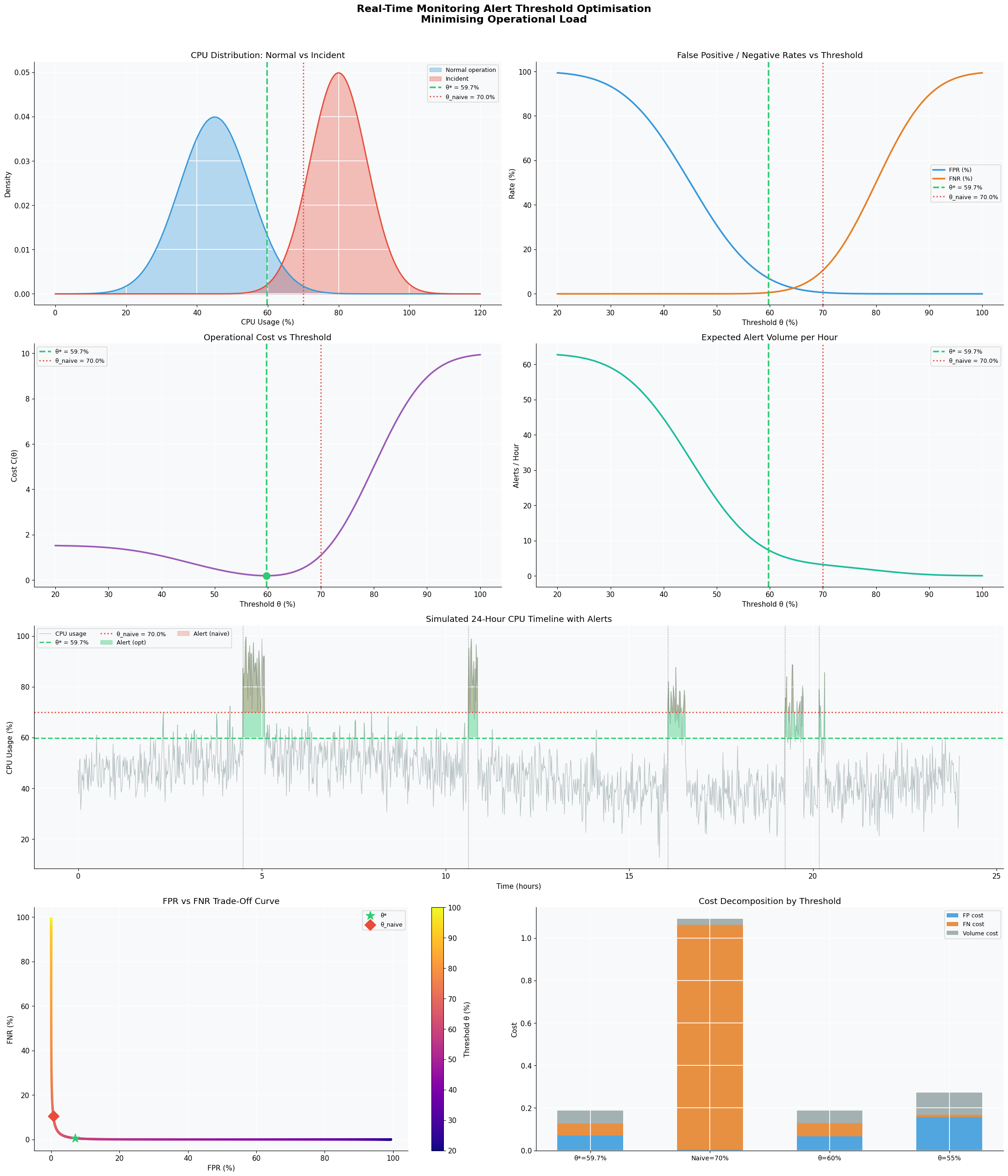
Figure 1 — 2D Dashboard (8 panels)

  • Top-left (CPU Distributions): The overlap region between the normal and incident distributions is where the threshold lives. Too far left = too many FP; too far right = too many missed incidents.
  • Top-right (FPR/FNR curves): Classic trade-off — as $\theta$ increases, FPR drops but FNR rises. The optimal point balances both weighted by $\lambda_{fp}$ and $\lambda_{fn}$.
  • Middle-left (Cost function): The bowl-shaped minimum clearly shows $\theta^* \approx 65%$. The naive threshold at 70% sits to the right, incurring higher missed-incident cost.
  • Middle-right (Alert volume): Alert volume drops exponentially as $\theta$ rises. High thresholds are quiet — but dangerously so.
  • Center (24-hour timeline): Green shading shows alerts fired by $\theta^*$; red shading shows the naive threshold’s alerts. Incident injection times are marked with dotted vertical lines.
  • Bottom-left (Trade-off curve): This is a parametric plot of FPR vs FNR as $\theta$ varies — analogous to an ROC curve. $\theta^*$ (star marker) lies closest to the ideal origin relative to the cost-weighted objective.
  • Bottom-right (Cost decomposition): Stacked bar chart comparing four thresholds. At $\theta^*$, the FN cost (orange) is well-controlled without inflating the FP cost (blue).

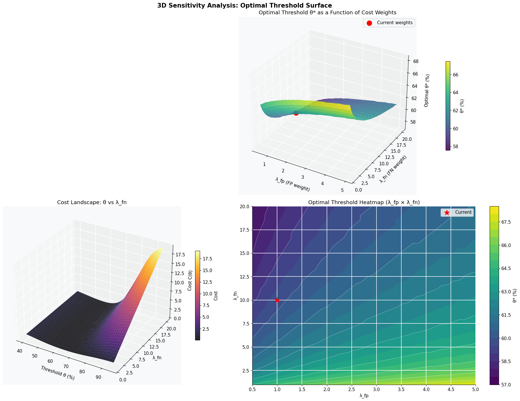
Figure 2 — 3D Sensitivity Analysis (4 panels)

  • Top (3D surface): Shows how $\theta^*$ shifts as the cost weights vary. When $\lambda_{fn} \gg \lambda_{fp}$ (bottom-right of the surface), the optimal threshold drops significantly — the system must become more sensitive to avoid missing costly incidents.
  • Bottom-left (Cost landscape): A 3D view of $C(\theta, \lambda_{fn})$, showing the valley floor that defines the optimal threshold at each weight setting.
  • Bottom-right (Heatmap): Top-down view of the surface — a practical tool for recalibrating thresholds when business priorities change (e.g., during peak sales season, $\lambda_{fn}$ should be raised, pushing $\theta^*$ down).

Results

=======================================================
  ALERT THRESHOLD OPTIMISATION RESULTS
=======================================================
  Optimal threshold  θ*  : 59.75%
  Minimum cost       C*  : 0.1879
  FPR at θ*              : 7.02%
  FNR at θ*              : 0.57%
  Alert volume/hr    V̄   : 7.32 alerts
  Cost at θ*-5pp         : 0.2813  (Δ=+0.0934)
  Cost at θ*+5pp         : 0.3443  (Δ=+0.1564)
=======================================================

[Figure 1 — 2D dashboard saved]

[Figure 2 — 3D sensitivity surface saved]

============================================================
  COMPARATIVE PERFORMANCE TABLE
============================================================
Metric                             θ*=59.7%      θ=70%      θ=60%
------------------------------------------------------------
FPR (%)                               7.02%      0.62%      6.68%
FNR (%)                               0.57%     10.56%      0.62%
Alerts/hr                              7.32       3.17       7.11
Total cost C(θ)                      0.1879     1.0891     0.1882
============================================================

Key Takeaways

The framework shows that alert threshold optimisation is a principled engineering problem, not guesswork. The three levers are:

  1. Accurately model your distributions — gather historical data to fit $\mu, \sigma$ for normal and incident states
  2. Quantify your cost weights — how many engineer-hours does a false alarm cost vs a missed P1 incident?
  3. Re-optimise dynamically — as traffic patterns change seasonally, $\mu$ and $\sigma$ drift, and $\theta^*$ should be updated automatically

For production systems, this pipeline can be run nightly on rolling 30-day CPU histograms to keep alert thresholds continuously calibrated — eliminating alert fatigue without sacrificing detection coverage.