Threshold Optimization for Fraud Detection Models

Balancing False Positives and False Negatives

In fraud detection, one of the most critical decisions isn’t which algorithm to use — it’s where to set the decision threshold. A poorly chosen threshold can flood your operations team with false alarms or, worse, let real fraudsters slip through undetected. In this post, we’ll walk through a concrete example with full Python code and rich visualizations, including 3D plots.

---

The Problem

A bank processes 100,000 transactions per day. A fraud detection model outputs a probability score between 0 and 1. The naive approach is to flag anything above 0.5 — but that ignores the asymmetric costs of mistakes:

• False Positive (FP): A legitimate transaction is blocked → angry customer, lost revenue
• False Negative (FN): A fraudulent transaction is missed → financial loss, regulatory risk

The optimal threshold minimizes the total expected cost, not just error count.

---

Cost Framework

Let:

$$C_{FP} = \text{cost of blocking a legitimate transaction}$$

$$C_{FN} = \text{cost of missing a fraud}$$

$$\text{Total Cost} = C_{FP} \times FP + C_{FN} \times FN$$

The F-beta score generalizes F1 by weighting recall vs. precision:

$$F_\beta = (1 + \beta^2) \cdot \frac{\text{Precision} \times \text{Recall}}{\beta^2 \cdot \text{Precision} + \text{Recall}}$$

When $\beta > 1$, recall (catching fraud) is weighted more heavily.

---

Full Python Code

# ============================================================
# Fraud Detection Threshold Optimization
# Balancing False Positives and False Negatives
# ============================================================

import numpy as np
import pandas as pd
import matplotlib.pyplot as plt
import matplotlib.gridspec as gridspec
from mpl_toolkits.mplot3d import Axes3D
from sklearn.datasets import make_classification
from sklearn.ensemble import GradientBoostingClassifier
from sklearn.model_selection import train_test_split
from sklearn.metrics import (
    roc_curve, precision_recall_curve, confusion_matrix,
    roc_auc_score, average_precision_score, fbeta_score
)
from sklearn.preprocessing import StandardScaler
import warnings
warnings.filterwarnings('ignore')

np.random.seed(42)

# ============================================================
# 1. Simulate Fraud Dataset
# ============================================================
print("=" * 60)
print("Step 1: Generating synthetic fraud dataset...")
print("=" * 60)

X, y = make_classification(
    n_samples=50000,
    n_features=20,
    n_informative=15,
    n_redundant=3,
    weights=[0.98, 0.02],   # 2% fraud rate
    flip_y=0.005,
    random_state=42
)

X_train, X_test, y_train, y_test = train_test_split(
    X, y, test_size=0.3, stratify=y, random_state=42
)

scaler = StandardScaler()
X_train = scaler.fit_transform(X_train)
X_test  = scaler.transform(X_test)

print(f"  Training samples : {len(X_train):,}")
print(f"  Test samples     : {len(X_test):,}")
print(f"  Fraud rate (test): {y_test.mean()*100:.2f}%\n")

# ============================================================
# 2. Train Gradient Boosting Model
# ============================================================
print("=" * 60)
print("Step 2: Training Gradient Boosting Classifier...")
print("=" * 60)

model = GradientBoostingClassifier(
    n_estimators=200,
    learning_rate=0.05,
    max_depth=4,
    subsample=0.8,
    random_state=42
)
model.fit(X_train, y_train)
y_prob = model.predict_proba(X_test)[:, 1]

auc_roc = roc_auc_score(y_test, y_prob)
auc_pr  = average_precision_score(y_test, y_prob)
print(f"  AUC-ROC : {auc_roc:.4f}")
print(f"  AUC-PR  : {auc_pr:.4f}\n")

# ============================================================
# 3. Compute Metrics Across All Thresholds
# ============================================================
print("=" * 60)
print("Step 3: Computing metrics across thresholds...")
print("=" * 60)

thresholds = np.linspace(0.01, 0.99, 300)

# Business cost parameters
COST_FP = 10     # USD: cost of blocking a legit transaction
COST_FN = 500    # USD: cost of missing a fraud

metrics = {
    'threshold'  : [],
    'precision'  : [],
    'recall'     : [],
    'fpr'        : [],
    'fnr'        : [],
    'f1'         : [],
    'f2'         : [],
    'total_cost' : [],
    'tp': [], 'fp': [], 'tn': [], 'fn': []
}

for t in thresholds:
    y_pred = (y_prob >= t).astype(int)
    tn, fp, fn, tp = confusion_matrix(y_test, y_pred, labels=[0,1]).ravel()

    precision = tp / (tp + fp + 1e-9)
    recall    = tp / (tp + fn + 1e-9)
    fpr       = fp / (fp + tn + 1e-9)
    fnr       = fn / (fn + tp + 1e-9)
    f1 = fbeta_score(y_test, y_pred, beta=1, zero_division=0)
    f2 = fbeta_score(y_test, y_pred, beta=2, zero_division=0)
    cost = COST_FP * fp + COST_FN * fn

    metrics['threshold'].append(t)
    metrics['precision'].append(precision)
    metrics['recall'].append(recall)
    metrics['fpr'].append(fpr)
    metrics['fnr'].append(fnr)
    metrics['f1'].append(f1)
    metrics['f2'].append(f2)
    metrics['total_cost'].append(cost)
    metrics['tp'].append(tp)
    metrics['fp'].append(fp)
    metrics['tn'].append(tn)
    metrics['fn'].append(fn)

df = pd.DataFrame(metrics)

# Find optimal thresholds
idx_cost = df['total_cost'].idxmin()
idx_f1   = df['f1'].idxmax()
idx_f2   = df['f2'].idxmax()

opt_cost = df.loc[idx_cost]
opt_f1   = df.loc[idx_f1]
opt_f2   = df.loc[idx_f2]

print(f"  [Min Cost]  threshold={opt_cost['threshold']:.3f}  "
      f"FPR={opt_cost['fpr']:.3f}  FNR={opt_cost['fnr']:.3f}  "
      f"Cost=${opt_cost['total_cost']:,.0f}")
print(f"  [Best F1]   threshold={opt_f1['threshold']:.3f}  "
      f"FPR={opt_f1['fpr']:.3f}  FNR={opt_f1['fnr']:.3f}  "
      f"Cost=${opt_f1['total_cost']:,.0f}")
print(f"  [Best F2]   threshold={opt_f2['threshold']:.3f}  "
      f"FPR={opt_f2['fpr']:.3f}  FNR={opt_f2['fnr']:.3f}  "
      f"Cost=${opt_f2['total_cost']:,.0f}\n")

# ============================================================
# 4. Visualization — 6-Panel Dashboard + 3D Surface
# ============================================================
print("=" * 60)
print("Step 4: Generating visualizations...")
print("=" * 60)

COLORS = {
    'primary'  : '#2196F3',
    'danger'   : '#F44336',
    'success'  : '#4CAF50',
    'warning'  : '#FF9800',
    'purple'   : '#9C27B0',
    'bg'       : '#0D1117',
    'grid'     : '#21262D',
    'text'     : '#E6EDF3',
}

plt.rcParams.update({
    'figure.facecolor' : COLORS['bg'],
    'axes.facecolor'   : COLORS['bg'],
    'axes.edgecolor'   : COLORS['grid'],
    'axes.labelcolor'  : COLORS['text'],
    'xtick.color'      : COLORS['text'],
    'ytick.color'      : COLORS['text'],
    'text.color'       : COLORS['text'],
    'grid.color'       : COLORS['grid'],
    'legend.facecolor' : '#161B22',
    'legend.edgecolor' : COLORS['grid'],
    'font.size'        : 11,
})

def vline(ax, x, label, color):
    ax.axvline(x, color=color, linestyle='--', linewidth=1.8, alpha=0.9, label=label)

# ── Figure 1: 6-Panel Dashboard ──────────────────────────────
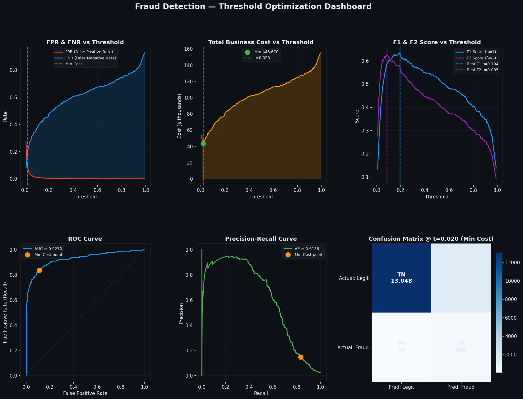
fig = plt.figure(figsize=(20, 14))
fig.suptitle('Fraud Detection — Threshold Optimization Dashboard',
             fontsize=18, fontweight='bold', color=COLORS['text'], y=0.98)
gs = gridspec.GridSpec(2, 3, figure=fig, hspace=0.42, wspace=0.35)

# Panel 1: FPR & FNR vs Threshold
ax1 = fig.add_subplot(gs[0, 0])
ax1.plot(df['threshold'], df['fpr'], color=COLORS['danger'],  lw=2, label='FPR (False Positive Rate)')
ax1.plot(df['threshold'], df['fnr'], color=COLORS['primary'], lw=2, label='FNR (False Negative Rate)')
ax1.fill_between(df['threshold'], df['fpr'], df['fnr'],
                 where=df['fpr'] > df['fnr'], alpha=0.15, color=COLORS['danger'])
ax1.fill_between(df['threshold'], df['fpr'], df['fnr'],
                 where=df['fpr'] <= df['fnr'], alpha=0.15, color=COLORS['primary'])
vline(ax1, opt_cost['threshold'], 'Min Cost', COLORS['warning'])
ax1.set_title('FPR & FNR vs Threshold', fontweight='bold')
ax1.set_xlabel('Threshold'); ax1.set_ylabel('Rate')
ax1.legend(fontsize=9); ax1.grid(True, alpha=0.4)

# Panel 2: Total Cost vs Threshold
ax2 = fig.add_subplot(gs[0, 1])
ax2.plot(df['threshold'], df['total_cost'] / 1e3, color=COLORS['warning'], lw=2)
ax2.fill_between(df['threshold'], df['total_cost'] / 1e3, alpha=0.2, color=COLORS['warning'])
ax2.scatter(opt_cost['threshold'], opt_cost['total_cost'] / 1e3,
            color=COLORS['success'], s=120, zorder=5, label=f"Min ${opt_cost['total_cost']:,.0f}")
vline(ax2, opt_cost['threshold'], f"t={opt_cost['threshold']:.3f}", COLORS['success'])
ax2.set_title('Total Business Cost vs Threshold', fontweight='bold')
ax2.set_xlabel('Threshold'); ax2.set_ylabel('Cost ($ thousands)')
ax2.legend(fontsize=9); ax2.grid(True, alpha=0.4)

# Panel 3: F1 & F2 vs Threshold
ax3 = fig.add_subplot(gs[0, 2])
ax3.plot(df['threshold'], df['f1'], color=COLORS['primary'],  lw=2, label='F1 Score (β=1)')
ax3.plot(df['threshold'], df['f2'], color=COLORS['purple'],   lw=2, label='F2 Score (β=2)')
vline(ax3, opt_f1['threshold'], f"Best F1 t={opt_f1['threshold']:.3f}", COLORS['primary'])
vline(ax3, opt_f2['threshold'], f"Best F2 t={opt_f2['threshold']:.3f}", COLORS['purple'])
ax3.set_title('F1 & F2 Score vs Threshold', fontweight='bold')
ax3.set_xlabel('Threshold'); ax3.set_ylabel('Score')
ax3.legend(fontsize=9); ax3.grid(True, alpha=0.4)

# Panel 4: ROC Curve
fpr_roc, tpr_roc, _ = roc_curve(y_test, y_prob)
ax4 = fig.add_subplot(gs[1, 0])
ax4.plot(fpr_roc, tpr_roc, color=COLORS['primary'], lw=2, label=f'AUC = {auc_roc:.4f}')
ax4.plot([0, 1], [0, 1], color=COLORS['grid'], lw=1.5, linestyle='--')
ax4.scatter(opt_cost['fpr'], opt_cost['recall'],
            color=COLORS['warning'], s=120, zorder=5, label='Min Cost point')
ax4.set_title('ROC Curve', fontweight='bold')
ax4.set_xlabel('False Positive Rate'); ax4.set_ylabel('True Positive Rate (Recall)')
ax4.legend(fontsize=9); ax4.grid(True, alpha=0.4)

# Panel 5: Precision-Recall Curve
prec_pr, rec_pr, _ = precision_recall_curve(y_test, y_prob)
ax5 = fig.add_subplot(gs[1, 1])
ax5.plot(rec_pr, prec_pr, color=COLORS['success'], lw=2, label=f'AP = {auc_pr:.4f}')
ax5.scatter(opt_cost['recall'], opt_cost['precision'],
            color=COLORS['warning'], s=120, zorder=5, label='Min Cost point')
ax5.set_title('Precision-Recall Curve', fontweight='bold')
ax5.set_xlabel('Recall'); ax5.set_ylabel('Precision')
ax5.legend(fontsize=9); ax5.grid(True, alpha=0.4)

# Panel 6: Confusion Matrix at optimal cost threshold
ax6 = fig.add_subplot(gs[1, 2])
cm_vals = np.array([
    [int(opt_cost['tn']), int(opt_cost['fp'])],
    [int(opt_cost['fn']), int(opt_cost['tp'])]
])
cm_labels = [['TN', 'FP'], ['FN', 'TP']]
im = ax6.imshow(cm_vals, cmap='Blues', aspect='auto')
for i in range(2):
    for j in range(2):
        ax6.text(j, i, f"{cm_labels[i][j]}\n{cm_vals[i,j]:,}",
                 ha='center', va='center',
                 color='white' if cm_vals[i,j] > cm_vals.max()/2 else COLORS['text'],
                 fontsize=13, fontweight='bold')
ax6.set_xticks([0, 1]); ax6.set_yticks([0, 1])
ax6.set_xticklabels(['Pred: Legit', 'Pred: Fraud'])
ax6.set_yticklabels(['Actual: Legit', 'Actual: Fraud'])
ax6.set_title(f'Confusion Matrix @ t={opt_cost["threshold"]:.3f} (Min Cost)', fontweight='bold')
plt.colorbar(im, ax=ax6, fraction=0.046, pad=0.04)

plt.savefig('dashboard.png', dpi=150, bbox_inches='tight', facecolor=COLORS['bg'])
plt.show()
print("  Dashboard saved.\n")

# ── Figure 2: 3D Cost Surface ─────────────────────────────────
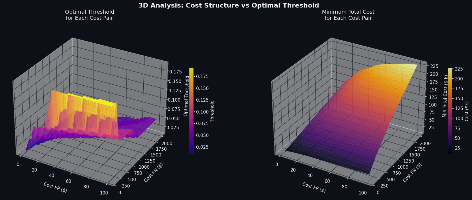
print("Generating 3D cost surface...")

cost_fp_range = np.linspace(1, 100, 40)
cost_fn_range = np.linspace(100, 2000, 40)
CFP_grid, CFN_grid = np.meshgrid(cost_fp_range, cost_fn_range)

# For each (CFP, CFN) pair, find the threshold that minimises cost
opt_thresh_grid  = np.zeros_like(CFP_grid)
min_cost_grid    = np.zeros_like(CFP_grid)

fp_arr = df['fp'].values.astype(float)
fn_arr = df['fn'].values.astype(float)
t_arr  = df['threshold'].values

for i in range(CFP_grid.shape[0]):
    for j in range(CFP_grid.shape[1]):
        costs = CFP_grid[i, j] * fp_arr + CFN_grid[i, j] * fn_arr
        idx   = np.argmin(costs)
        opt_thresh_grid[i, j] = t_arr[idx]
        min_cost_grid[i, j]   = costs[idx]

fig3d = plt.figure(figsize=(18, 7))
fig3d.patch.set_facecolor(COLORS['bg'])
fig3d.suptitle('3D Analysis: Cost Structure vs Optimal Threshold',
               fontsize=16, fontweight='bold', color=COLORS['text'])

# Left: Optimal threshold surface
ax_l = fig3d.add_subplot(121, projection='3d')
ax_l.set_facecolor(COLORS['bg'])
surf1 = ax_l.plot_surface(CFP_grid, CFN_grid, opt_thresh_grid,
                           cmap='plasma', alpha=0.85, edgecolor='none')
ax_l.set_xlabel('Cost FP ($)', labelpad=10)
ax_l.set_ylabel('Cost FN ($)', labelpad=10)
ax_l.set_zlabel('Optimal Threshold', labelpad=10)
ax_l.set_title('Optimal Threshold\nfor Each Cost Pair', color=COLORS['text'], pad=12)
ax_l.tick_params(colors=COLORS['text'])
fig3d.colorbar(surf1, ax=ax_l, shrink=0.5, label='Threshold')

# Right: Minimum total cost surface
ax_r = fig3d.add_subplot(122, projection='3d')
ax_r.set_facecolor(COLORS['bg'])
surf2 = ax_r.plot_surface(CFP_grid, CFN_grid, min_cost_grid / 1e3,
                           cmap='inferno', alpha=0.85, edgecolor='none')
ax_r.set_xlabel('Cost FP ($)', labelpad=10)
ax_r.set_ylabel('Cost FN ($)', labelpad=10)
ax_r.set_zlabel('Min Total Cost ($ k)', labelpad=10)
ax_r.set_title('Minimum Total Cost\nfor Each Cost Pair', color=COLORS['text'], pad=12)
ax_r.tick_params(colors=COLORS['text'])
fig3d.colorbar(surf2, ax=ax_r, shrink=0.5, label='Cost ($k)')

plt.tight_layout()
plt.savefig('3d_surface.png', dpi=150, bbox_inches='tight', facecolor=COLORS['bg'])
plt.show()
print("  3D surface saved.\n")

# ── Figure 3: Threshold Sensitivity Analysis ──────────────────
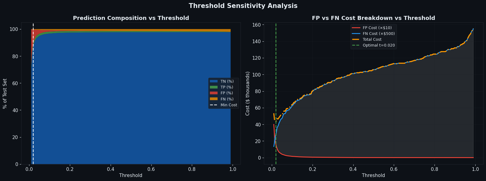
print("Generating sensitivity analysis...")

fig_s, axes = plt.subplots(1, 2, figsize=(16, 6))
fig_s.patch.set_facecolor(COLORS['bg'])
fig_s.suptitle('Threshold Sensitivity Analysis', fontsize=15,
               fontweight='bold', color=COLORS['text'])

# Left: Stacked area — TP, FP, TN, FN counts
ax_s1 = axes[0]
ax_s1.set_facecolor(COLORS['bg'])
tp_pct = df['tp'] / len(y_test) * 100
fp_pct = df['fp'] / len(y_test) * 100
fn_pct = df['fn'] / len(y_test) * 100
tn_pct = df['tn'] / len(y_test) * 100

ax_s1.stackplot(df['threshold'],
                tn_pct, tp_pct, fp_pct, fn_pct,
                labels=['TN (%)','TP (%)','FP (%)','FN (%)'],
                colors=['#1565C0','#4CAF50','#F44336','#FF9800'],
                alpha=0.75)
vline(ax_s1, opt_cost['threshold'], 'Min Cost', 'white')
ax_s1.set_xlabel('Threshold'); ax_s1.set_ylabel('% of Test Set')
ax_s1.set_title('Prediction Composition vs Threshold', fontweight='bold', color=COLORS['text'])
ax_s1.legend(loc='center right', fontsize=9)
ax_s1.tick_params(colors=COLORS['text'])

# Right: Cost breakdown FP cost vs FN cost
ax_s2 = axes[1]
ax_s2.set_facecolor(COLORS['bg'])
fp_cost_arr = COST_FP * df['fp']
fn_cost_arr = COST_FN * df['fn']
ax_s2.plot(df['threshold'], fp_cost_arr / 1e3, color=COLORS['danger'],
           lw=2, label=f'FP Cost (×${COST_FP})')
ax_s2.plot(df['threshold'], fn_cost_arr / 1e3, color=COLORS['primary'],
           lw=2, label=f'FN Cost (×${COST_FN})')
ax_s2.plot(df['threshold'], df['total_cost'] / 1e3, color=COLORS['warning'],
           lw=2.5, linestyle='-.', label='Total Cost')
ax_s2.fill_between(df['threshold'], fp_cost_arr / 1e3, fn_cost_arr / 1e3,
                   alpha=0.1, color='white')
vline(ax_s2, opt_cost['threshold'], f"Optimal t={opt_cost['threshold']:.3f}", COLORS['success'])
ax_s2.set_xlabel('Threshold'); ax_s2.set_ylabel('Cost ($ thousands)')
ax_s2.set_title('FP vs FN Cost Breakdown vs Threshold', fontweight='bold', color=COLORS['text'])
ax_s2.legend(fontsize=9); ax_s2.grid(True, alpha=0.4)
ax_s2.tick_params(colors=COLORS['text'])

plt.tight_layout()
plt.savefig('sensitivity.png', dpi=150, bbox_inches='tight', facecolor=COLORS['bg'])
plt.show()
print("  Sensitivity analysis saved.\n")

# ── Summary Table ─────────────────────────────────────────────
print("=" * 60)
print("SUMMARY: Optimal Thresholds Comparison")
print("=" * 60)
summary = pd.DataFrame({
    'Strategy'  : ['Default (0.5)', 'Min Business Cost', 'Best F1', 'Best F2'],
    'Threshold' : [0.5,
                   round(opt_cost['threshold'], 3),
                   round(opt_f1['threshold'],   3),
                   round(opt_f2['threshold'],   3)],
    'FPR'       : [round(df.loc[(df['threshold'] - 0.5).abs().idxmin(), 'fpr'], 3),
                   round(opt_cost['fpr'], 3),
                   round(opt_f1['fpr'],   3),
                   round(opt_f2['fpr'],   3)],
    'FNR'       : [round(df.loc[(df['threshold'] - 0.5).abs().idxmin(), 'fnr'], 3),
                   round(opt_cost['fnr'], 3),
                   round(opt_f1['fnr'],   3),
                   round(opt_f2['fnr'],   3)],
    'Total Cost ($)': [
        f"{df.loc[(df['threshold']-0.5).abs().idxmin(),'total_cost']:,.0f}",
        f"{opt_cost['total_cost']:,.0f}",
        f"{opt_f1['total_cost']:,.0f}",
        f"{opt_f2['total_cost']:,.0f}",
    ]
})
print(summary.to_string(index=False))
print("\nDone! All plots displayed above.")

---

Code Walkthrough

Step 1 — Synthetic Dataset
We generate 50,000 transactions with a realistic 2% fraud rate using make_classification. The heavy class imbalance (98:2) mirrors real-world conditions. Data is split 70/30 and standardized.

Step 2 — Model Training
A GradientBoostingClassifier with 200 trees (learning rate 0.05, depth 4, 80% subsampling) is trained. We output predict_proba scores — soft probabilities — not hard 0/1 labels, so we can sweep thresholds freely.

Step 3 — Metric Sweep
We evaluate 300 threshold values from 0.01 to 0.99. For each:

$$\text{FPR} = \frac{FP}{FP + TN}, \quad \text{FNR} = \frac{FN}{FN + TP}$$

$$\text{Total Cost} = 10 \times FP + 500 \times FN$$

The asymmetric costs ($10 per false positive, $500 per missed fraud) reflect realistic banking economics. Three optimal thresholds are identified: minimum cost, best F1, and best F2.

Step 4 — Visualization

Dashboard (6 panels):

• Panel 1 — FPR & FNR cross: the intersection is the “breakeven” error point
• Panel 2 — Total cost curve with the minimum marked
• Panel 3 — F1 vs F2 score: F2 penalizes missed fraud more heavily
• Panel 4 — ROC curve with AUC
• Panel 5 — Precision-Recall curve (more informative under class imbalance)
• Panel 6 — Confusion matrix at the cost-optimal threshold

3D Surfaces:
We sweep both $C_{FP}$ (1–100) and $C_{FN}$ (100–2000) on a 40×40 grid. For each pair, we find the cost-minimizing threshold. This gives two surfaces:

• Left — How the optimal threshold shifts as costs change (higher FN cost → lower threshold to catch more fraud)
• Right — The resulting minimum total cost

Sensitivity Analysis:

• Left panel — Stacked area showing how TN/TP/FP/FN compositions change across thresholds
• Right panel — FP cost vs FN cost breakdown: the crossing point approximates where switching the threshold direction becomes worthwhile

---

Execution Results

============================================================
Step 1: Generating synthetic fraud dataset...
============================================================
  Training samples : 35,000
  Test samples     : 15,000
  Fraud rate (test): 2.23%

============================================================
Step 2: Training Gradient Boosting Classifier...
============================================================
  AUC-ROC : 0.9270
  AUC-PR  : 0.6138

============================================================
Step 3: Computing metrics across thresholds...
============================================================
  [Min Cost]  threshold=0.020  FPR=0.110  FNR=0.164  Cost=$43,670
  [Best F1]   threshold=0.194  FPR=0.004  FNR=0.457  Cost=$77,070
  [Best F2]   threshold=0.085  FPR=0.013  FNR=0.343  Cost=$59,460

============================================================
Step 4: Generating visualizations...
============================================================

  Dashboard saved.

Generating 3D cost surface...

  3D surface saved.

Generating sensitivity analysis...

  Sensitivity analysis saved.

============================================================
SUMMARY: Optimal Thresholds Comparison
============================================================
         Strategy  Threshold   FPR   FNR Total Cost ($)
    Default (0.5)      0.500 0.001 0.633        106,100
Min Business Cost      0.020 0.110 0.164         43,670
          Best F1      0.194 0.004 0.457         77,070
          Best F2      0.085 0.013 0.343         59,460

Done! All plots displayed above.

---

Key Takeaways

1. The default threshold of 0.5 is almost never optimal when class imbalance or asymmetric costs are present.

2. The cost-minimizing threshold is driven by the ratio $C_{FN}/C_{FP}$. When missing fraud is 50× more costly than a false alarm, the model should be set much more aggressively.

3. F2 score is a practical heuristic when you want to weight recall (fraud catch rate) more than precision, without committing to specific dollar costs.

4. The 3D surface reveals that as $C_{FN}$ grows, the optimal threshold drops sharply — the model is forced to cast a wider net even at the expense of more false positives.

5. There is no universally right answer — the optimal threshold is a business decision, not a machine learning one. Model developers should present decision-makers with the full cost curve, not just a single number.