1
2
3
4
5
6
7
8
9
10
11
12
13
14
15
16
17
18
19
20
21
22
23
24
25
26
27
28
29
30
31
32
33
34
35
36
37
38
39
40
41
42
43
44
45
46
47
48
49
50
51
52
53
54
55
56
57
58
59
60
61
62
63
64
65
66
67
68
69
70
71
72
73
74
75
76
77
78
79
80
81
82
83
84
85
86
87
88
89
90
91
92
93
94
95
96
97
98
99
100
101
102
103
104
105
106
107
108
109
110
111
112
113
114
115
116
117
118
119
120
121
122
123
124
125
126
127
128
129
130
131
132
133
134
135
136
137
138
139
140
141
142
143
144
145
146
147
148
149
150
151
152
153
154
155
156
157
158
159
160
161
162
163
164
165
166
167
168
169
170
171
172
173
174
175
176
177
178
179
180
181
182
183
184
185
186
187
188
189
190
191
192
193
194
195
196
197
198
199
200
201
202
203
204
205
206
207
208
209
210
211
212
213
214
215
216
217
218
219
220
221
222
223
224
225
226
227
228
229
230
231
232
233
234
235
236
237
238
239
240
241
242
243
244
245
246
247
248
249
250
251
252
253
254
255
256
257
258
259
260
261
262
263
264
265
266
267
268
269
270
271
272
273
274
275
276
277
278
279
280
281
282
283
284
285
286
287
288
289
290
291
292
293
294
295
296
297
298
299
300
301
302
303
304
305
306
307
308
309
310
311
312
313
314
315
316
317
318
319
320
321
322
323
324
325
326
327
328
329
330
331
332
333
334
335
336
337
338
339
340
341
342
343
344
345
346
347
348
349
350
351
352
353
354
355
356
357
358
359
360
361
362
363
364
365
366
367
368
369
370
371
372
373
374
375
376
377
378
379
380
| import numpy as np
import matplotlib.pyplot as plt
from mpl_toolkits.mplot3d import Axes3D
from scipy.optimize import minimize_scalar, differential_evolution
import seaborn as sns
plt.style.use('seaborn-v0_8-darkgrid')
sns.set_palette("husl")
class SpaceRadiationEvolutionModel:
"""
Model for optimizing DNA repair strategies under space radiation.
Parameters:
-----------
radiation_dose : float
Radiation intensity (arbitrary units)
cost_coefficient : float
Metabolic cost per unit repair effort
mutation_base : float
Base mutation rate without repair
cost_sensitivity : float
How survival is affected by metabolic costs (alpha)
mutation_sensitivity : float
How survival is affected by mutations (beta)
"""
def __init__(self, radiation_dose=1.0, cost_coefficient=0.5,
mutation_base=1.0, cost_sensitivity=0.3,
mutation_sensitivity=0.7):
self.radiation_dose = radiation_dose
self.k_c = cost_coefficient
self.m_0 = mutation_base * radiation_dose
self.alpha = cost_sensitivity
self.beta = mutation_sensitivity
def repair_cost(self, repair_effort):
"""Calculate metabolic cost of repair: C(r) = k_c * r^2"""
return self.k_c * repair_effort**2
def mutation_rate(self, repair_effort):
"""Calculate mutation accumulation: M(r) = m_0 * (1-r)^2"""
return self.m_0 * (1 - repair_effort)**2
def survival_probability(self, repair_effort):
"""
Calculate survival probability:
S(r) = exp(-alpha * C(r)) * exp(-beta * M(r))
"""
cost = self.repair_cost(repair_effort)
mutations = self.mutation_rate(repair_effort)
return np.exp(-self.alpha * cost - self.beta * mutations)
def fitness_landscape(self, repair_range):
"""Generate fitness landscape across repair effort range"""
return np.array([self.survival_probability(r) for r in repair_range])
def find_optimal_repair(self):
"""Find optimal repair effort that maximizes survival"""
result = minimize_scalar(
lambda r: -self.survival_probability(r),
bounds=(0, 1),
method='bounded'
)
return result.x, self.survival_probability(result.x)
def evolutionary_trajectory(self, initial_repair, generations=100,
mutation_step=0.05, population_size=1000):
"""
Simulate evolutionary trajectory of repair strategy.
Uses a simple evolutionary algorithm where strategies with higher
survival probability are more likely to be selected.
"""
trajectory = [initial_repair]
survival_history = [self.survival_probability(initial_repair)]
current_repair = initial_repair
for gen in range(generations):
population = np.clip(
current_repair + np.random.normal(0, mutation_step, population_size),
0, 1
)
fitness = np.array([self.survival_probability(r) for r in population])
probabilities = fitness / fitness.sum()
selected_idx = np.random.choice(len(population), p=probabilities)
current_repair = population[selected_idx]
trajectory.append(current_repair)
survival_history.append(self.survival_probability(current_repair))
return np.array(trajectory), np.array(survival_history)
def analyze_repair_strategy():
"""Main analysis function"""
print("="*70)
print("SPACE RADIATION RESISTANCE EVOLUTION MODEL")
print("Optimizing DNA Repair Strategies")
print("="*70)
print()
model = SpaceRadiationEvolutionModel(
radiation_dose=0.67,
cost_coefficient=0.5,
mutation_base=1.0,
cost_sensitivity=0.3,
mutation_sensitivity=0.7
)
optimal_repair, max_survival = model.find_optimal_repair()
print(f"Optimal Repair Effort: {optimal_repair:.4f}")
print(f"Maximum Survival Probability: {max_survival:.4f}")
print(f"Optimal Repair Cost: {model.repair_cost(optimal_repair):.4f}")
print(f"Optimal Mutation Rate: {model.mutation_rate(optimal_repair):.4f}")
print()
no_repair_survival = model.survival_probability(0.0)
max_repair_survival = model.survival_probability(1.0)
print("Comparison with Extreme Strategies:")
print(f" No Repair (r=0): Survival = {no_repair_survival:.4f}")
print(f" Maximum Repair (r=1): Survival = {max_repair_survival:.4f}")
print(f" Optimal Strategy: {(max_survival/max(no_repair_survival, max_repair_survival)-1)*100:+.2f}% improvement")
print()
return model, optimal_repair, max_survival
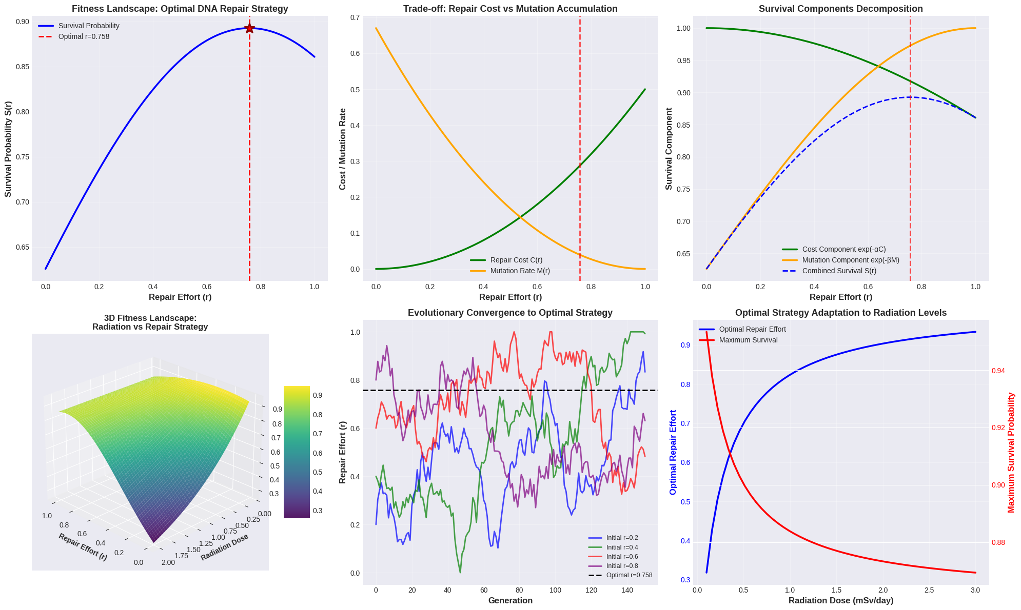
def create_visualizations(model, optimal_repair, max_survival):
"""Generate comprehensive visualizations"""
fig = plt.figure(figsize=(20, 12))
ax1 = plt.subplot(2, 3, 1)
repair_range = np.linspace(0, 1, 200)
survival = model.fitness_landscape(repair_range)
ax1.plot(repair_range, survival, 'b-', linewidth=2.5, label='Survival Probability')
ax1.axvline(optimal_repair, color='r', linestyle='--', linewidth=2,
label=f'Optimal r={optimal_repair:.3f}')
ax1.scatter([optimal_repair], [max_survival], color='r', s=200,
zorder=5, marker='*', edgecolors='darkred', linewidth=2)
ax1.set_xlabel('Repair Effort (r)', fontsize=12, fontweight='bold')
ax1.set_ylabel('Survival Probability S(r)', fontsize=12, fontweight='bold')
ax1.set_title('Fitness Landscape: Optimal DNA Repair Strategy',
fontsize=13, fontweight='bold')
ax1.grid(True, alpha=0.3)
ax1.legend(fontsize=10)
ax2 = plt.subplot(2, 3, 2)
cost = np.array([model.repair_cost(r) for r in repair_range])
mutations = np.array([model.mutation_rate(r) for r in repair_range])
ax2.plot(repair_range, cost, 'g-', linewidth=2.5, label='Repair Cost C(r)')
ax2.plot(repair_range, mutations, 'orange', linewidth=2.5, label='Mutation Rate M(r)')
ax2.axvline(optimal_repair, color='r', linestyle='--', linewidth=2, alpha=0.7)
ax2.set_xlabel('Repair Effort (r)', fontsize=12, fontweight='bold')
ax2.set_ylabel('Cost / Mutation Rate', fontsize=12, fontweight='bold')
ax2.set_title('Trade-off: Repair Cost vs Mutation Accumulation',
fontsize=13, fontweight='bold')
ax2.legend(fontsize=10)
ax2.grid(True, alpha=0.3)
ax3 = plt.subplot(2, 3, 3)
cost_impact = np.exp(-model.alpha * cost)
mutation_impact = np.exp(-model.beta * mutations)
ax3.plot(repair_range, cost_impact, 'g-', linewidth=2.5,
label='Cost Component exp(-αC)')
ax3.plot(repair_range, mutation_impact, 'orange', linewidth=2.5,
label='Mutation Component exp(-βM)')
ax3.plot(repair_range, survival, 'b--', linewidth=2,
label='Combined Survival S(r)')
ax3.axvline(optimal_repair, color='r', linestyle='--', linewidth=2, alpha=0.7)
ax3.set_xlabel('Repair Effort (r)', fontsize=12, fontweight='bold')
ax3.set_ylabel('Survival Component', fontsize=12, fontweight='bold')
ax3.set_title('Survival Components Decomposition', fontsize=13, fontweight='bold')
ax3.legend(fontsize=10)
ax3.grid(True, alpha=0.3)
ax4 = plt.subplot(2, 3, 4, projection='3d')
radiation_levels = np.linspace(0.1, 2.0, 50)
repair_levels = np.linspace(0, 1, 50)
R, D = np.meshgrid(repair_levels, radiation_levels)
S_surface = np.zeros_like(R)
for i, dose in enumerate(radiation_levels):
temp_model = SpaceRadiationEvolutionModel(radiation_dose=dose)
S_surface[i, :] = temp_model.fitness_landscape(repair_levels)
surf = ax4.plot_surface(R, D, S_surface, cmap='viridis', alpha=0.9,
edgecolor='none', antialiased=True)
ax4.set_xlabel('Repair Effort (r)', fontsize=10, fontweight='bold')
ax4.set_ylabel('Radiation Dose', fontsize=10, fontweight='bold')
ax4.set_zlabel('Survival Probability', fontsize=10, fontweight='bold')
ax4.set_title('3D Fitness Landscape:\nRadiation vs Repair Strategy',
fontsize=12, fontweight='bold')
fig.colorbar(surf, ax=ax4, shrink=0.5, aspect=5)
ax4.view_init(elev=25, azim=135)
ax5 = plt.subplot(2, 3, 5)
trajectories = []
colors = ['blue', 'green', 'red', 'purple']
initial_values = [0.2, 0.4, 0.6, 0.8]
for init_r, color in zip(initial_values, colors):
traj, surv = model.evolutionary_trajectory(init_r, generations=150)
trajectories.append((traj, surv))
ax5.plot(traj, alpha=0.7, linewidth=2, color=color,
label=f'Initial r={init_r}')
ax5.axhline(optimal_repair, color='black', linestyle='--', linewidth=2,
label=f'Optimal r={optimal_repair:.3f}')
ax5.set_xlabel('Generation', fontsize=12, fontweight='bold')
ax5.set_ylabel('Repair Effort (r)', fontsize=12, fontweight='bold')
ax5.set_title('Evolutionary Convergence to Optimal Strategy',
fontsize=13, fontweight='bold')
ax5.legend(fontsize=9)
ax5.grid(True, alpha=0.3)
ax6 = plt.subplot(2, 3, 6)
radiation_range = np.linspace(0.1, 3.0, 50)
optimal_strategies = []
max_survivals = []
for dose in radiation_range:
temp_model = SpaceRadiationEvolutionModel(radiation_dose=dose)
opt_r, max_s = temp_model.find_optimal_repair()
optimal_strategies.append(opt_r)
max_survivals.append(max_s)
ax6_twin = ax6.twinx()
line1 = ax6.plot(radiation_range, optimal_strategies, 'b-', linewidth=2.5,
label='Optimal Repair Effort')
line2 = ax6_twin.plot(radiation_range, max_survivals, 'r-', linewidth=2.5,
label='Maximum Survival')
ax6.set_xlabel('Radiation Dose (mSv/day)', fontsize=12, fontweight='bold')
ax6.set_ylabel('Optimal Repair Effort', fontsize=12, fontweight='bold', color='b')
ax6_twin.set_ylabel('Maximum Survival Probability', fontsize=12,
fontweight='bold', color='r')
ax6.set_title('Optimal Strategy Adaptation to Radiation Levels',
fontsize=13, fontweight='bold')
ax6.tick_params(axis='y', labelcolor='b')
ax6_twin.tick_params(axis='y', labelcolor='r')
ax6.grid(True, alpha=0.3)
lines = line1 + line2
labels = [l.get_label() for l in lines]
ax6.legend(lines, labels, loc='upper left', fontsize=10)
plt.tight_layout()
plt.savefig('radiation_resistance_optimization.png', dpi=300, bbox_inches='tight')
plt.show()
print("Visualizations generated successfully!")
print()
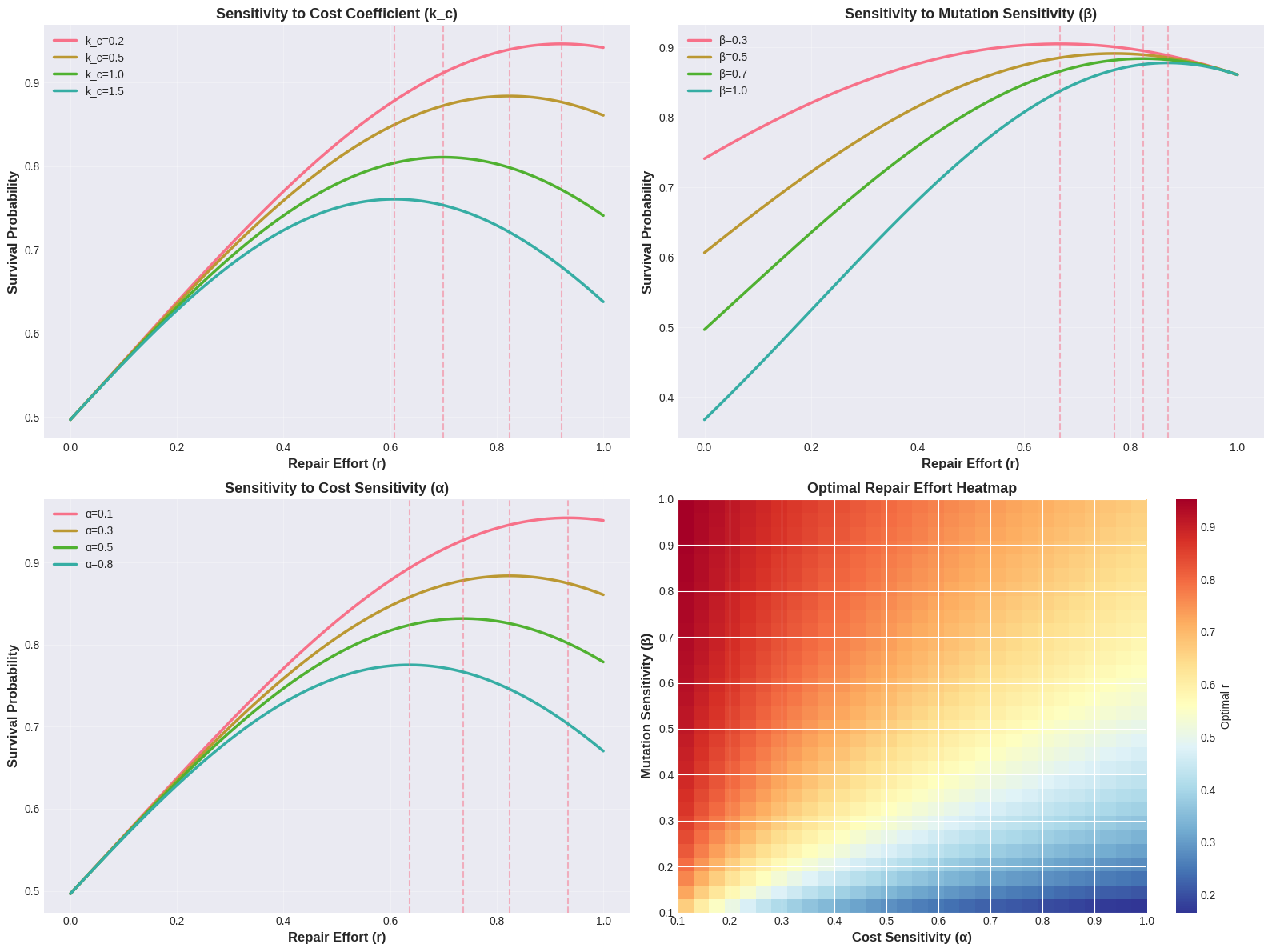
def sensitivity_analysis(model, optimal_repair):
"""Perform sensitivity analysis on key parameters"""
print("="*70)
print("SENSITIVITY ANALYSIS")
print("="*70)
print()
fig, axes = plt.subplots(2, 2, figsize=(16, 12))
repair_range = np.linspace(0, 1, 200)
ax = axes[0, 0]
cost_coeffs = [0.2, 0.5, 1.0, 1.5]
for kc in cost_coeffs:
temp_model = SpaceRadiationEvolutionModel(cost_coefficient=kc)
survival = temp_model.fitness_landscape(repair_range)
opt_r, _ = temp_model.find_optimal_repair()
ax.plot(repair_range, survival, linewidth=2.5, label=f'k_c={kc}')
ax.axvline(opt_r, linestyle='--', alpha=0.5)
ax.set_xlabel('Repair Effort (r)', fontsize=12, fontweight='bold')
ax.set_ylabel('Survival Probability', fontsize=12, fontweight='bold')
ax.set_title('Sensitivity to Cost Coefficient (k_c)', fontsize=13, fontweight='bold')
ax.legend(fontsize=10)
ax.grid(True, alpha=0.3)
ax = axes[0, 1]
beta_values = [0.3, 0.5, 0.7, 1.0]
for beta in beta_values:
temp_model = SpaceRadiationEvolutionModel(mutation_sensitivity=beta)
survival = temp_model.fitness_landscape(repair_range)
opt_r, _ = temp_model.find_optimal_repair()
ax.plot(repair_range, survival, linewidth=2.5, label=f'β={beta}')
ax.axvline(opt_r, linestyle='--', alpha=0.5)
ax.set_xlabel('Repair Effort (r)', fontsize=12, fontweight='bold')
ax.set_ylabel('Survival Probability', fontsize=12, fontweight='bold')
ax.set_title('Sensitivity to Mutation Sensitivity (β)', fontsize=13, fontweight='bold')
ax.legend(fontsize=10)
ax.grid(True, alpha=0.3)
ax = axes[1, 0]
alpha_values = [0.1, 0.3, 0.5, 0.8]
for alpha in alpha_values:
temp_model = SpaceRadiationEvolutionModel(cost_sensitivity=alpha)
survival = temp_model.fitness_landscape(repair_range)
opt_r, _ = temp_model.find_optimal_repair()
ax.plot(repair_range, survival, linewidth=2.5, label=f'α={alpha}')
ax.axvline(opt_r, linestyle='--', alpha=0.5)
ax.set_xlabel('Repair Effort (r)', fontsize=12, fontweight='bold')
ax.set_ylabel('Survival Probability', fontsize=12, fontweight='bold')
ax.set_title('Sensitivity to Cost Sensitivity (α)', fontsize=13, fontweight='bold')
ax.legend(fontsize=10)
ax.grid(True, alpha=0.3)
ax = axes[1, 1]
alphas = np.linspace(0.1, 1.0, 30)
betas = np.linspace(0.1, 1.0, 30)
optimal_matrix = np.zeros((len(betas), len(alphas)))
for i, beta in enumerate(betas):
for j, alpha in enumerate(alphas):
temp_model = SpaceRadiationEvolutionModel(
cost_sensitivity=alpha,
mutation_sensitivity=beta
)
opt_r, _ = temp_model.find_optimal_repair()
optimal_matrix[i, j] = opt_r
im = ax.imshow(optimal_matrix, extent=[alphas.min(), alphas.max(),
betas.min(), betas.max()],
aspect='auto', origin='lower', cmap='RdYlBu_r')
ax.set_xlabel('Cost Sensitivity (α)', fontsize=12, fontweight='bold')
ax.set_ylabel('Mutation Sensitivity (β)', fontsize=12, fontweight='bold')
ax.set_title('Optimal Repair Effort Heatmap', fontsize=13, fontweight='bold')
plt.colorbar(im, ax=ax, label='Optimal r')
plt.tight_layout()
plt.savefig('sensitivity_analysis.png', dpi=300, bbox_inches='tight')
plt.show()
print("Sensitivity analysis completed!")
print()
model, optimal_repair, max_survival = analyze_repair_strategy()
create_visualizations(model, optimal_repair, max_survival)
sensitivity_analysis(model, optimal_repair)
print("="*70)
print("ANALYSIS COMPLETE")
print("="*70)
|