Optimizing Capital Allocation in Financial Institutions

Balancing Risk-Weighted Assets


Capital allocation is one of the most critical challenges facing banks and financial institutions. Regulators require banks to hold sufficient capital against their risk-weighted assets (RWA), while shareholders demand maximum returns. How do you find the sweet spot? Let’s solve this with a concrete example using Python.


The Problem

Consider a bank with €500 billion in total capital that must allocate across 5 business lines:

Business Line Expected Return Risk Weight Min Allocation Max Allocation
Retail Banking 8% 35% €30B €150B
Corporate Lending 12% 100% €20B €120B
Trading 18% 200% €10B €80B
Mortgages 6% 50% €40B €200B
SME Lending 14% 75% €15B €100B

Regulatory constraint (Basel III): Total Risk-Weighted Assets must not exceed €400 billion, and the Capital Adequacy Ratio (CAR) must be ≥ 8%.


Mathematical Formulation

Let $x_i$ be the capital allocated to business line $i$.

Objective — Maximize total return:

$$\max \sum_{i=1}^{n} r_i \cdot x_i$$

Subject to:

$$\sum_{i=1}^{n} x_i = C_{\text{total}} \quad \text{(total capital constraint)}$$

$$\sum_{i=1}^{n} w_i \cdot x_i \leq \text{RWA}_{\max} \quad \text{(RWA constraint)}$$

$$\frac{C_{\text{total}}}{\sum_{i=1}^{n} w_i \cdot x_i} \geq \text{CAR}_{\min} \quad \text{(Capital Adequacy Ratio)}$$

$$x_i^{\min} \leq x_i \leq x_i^{\max} \quad \text{(business line bounds)}$$

Return on Risk-Weighted Assets (RoRWA):

$$\text{RoRWA}_i = \frac{r_i}{w_i}$$

This is the key efficiency metric — return per unit of regulatory capital consumed.


Python Solution

1
2
3
4
5
6
7
8
9
10
11
12
13
14
15
16
17
18
19
20
21
22
23
24
25
26
27
28
29
30
31
32
33
34
35
36
37
38
39
40
41
42
43
44
45
46
47
48
49
50
51
52
53
54
55
56
57
58
59
60
61
62
63
64
65
66
67
68
69
70
71
72
73
74
75
76
77
78
79
80
81
82
83
84
85
86
87
88
89
90
91
92
93
94
95
96
97
98
99
100
101
102
103
104
105
106
107
108
109
110
111
112
113
114
115
116
117
118
119
120
121
122
123
124
125
126
127
128
129
130
131
132
133
134
135
136
137
138
139
140
141
142
143
144
145
146
147
148
149
150
151
152
153
154
155
156
157
158
159
160
161
162
163
164
165
166
167
168
169
170
171
172
173
174
175
176
177
178
179
180
181
182
183
184
185
186
187
188
189
190
191
192
193
194
195
196
197
198
199
200
201
202
203
204
205
206
207
208
209
210
211
212
213
214
215
216
217
218
219
220
221
222
223
224
225
226
227
228
229
230
231
232
233
234
235
236
237
238
239
240
241
242
243
244
245
246
247
248
249
250
251
252
253
254
255
256
257
258
259
260
261
262
263
# ============================================================
# Capital Allocation Optimization for Financial Institutions
# Balancing Return vs. Risk-Weighted Assets (RWA) — Basel III
# ============================================================

import numpy as np
import pandas as pd
import matplotlib.pyplot as plt
import matplotlib.patches as mpatches
from matplotlib.gridspec import GridSpec
from scipy.optimize import linprog, minimize
from mpl_toolkits.mplot3d import Axes3D
from matplotlib import cm
import warnings
warnings.filterwarnings('ignore')

# --------------------------------------------------
# 1. PROBLEM PARAMETERS
# --------------------------------------------------
business_lines = ['Retail\nBanking', 'Corporate\nLending', 'Trading',
'Mortgages', 'SME\nLending']
labels_clean = ['Retail Banking', 'Corporate Lending', 'Trading',
'Mortgages', 'SME Lending']

returns = np.array([0.08, 0.12, 0.18, 0.06, 0.14]) # expected return rates
risk_weights = np.array([0.35, 1.00, 2.00, 0.50, 0.75]) # Basel III risk weights
x_min = np.array([30, 20, 10, 40, 15], dtype=float) # €B floor
x_max = np.array([150, 120, 80, 200, 100], dtype=float) # €B ceiling

TOTAL_CAPITAL = 500.0 # €B
RWA_MAX = 400.0 # €B (regulatory ceiling)
CAR_MIN = 0.08 # 8% minimum capital adequacy ratio
n = len(returns)

# RoRWA — efficiency metric
rorwa = returns / risk_weights

print("=" * 60)
print(" BUSINESS LINE PARAMETERS")
print("=" * 60)
df_params = pd.DataFrame({
'Business Line' : labels_clean,
'Return (%)' : returns * 100,
'Risk Weight (%)': risk_weights * 100,
'RoRWA (%)' : rorwa * 100,
'Min (€B)' : x_min,
'Max (€B)' : x_max,
})
print(df_params.to_string(index=False))


# --------------------------------------------------
# 2. LINEAR PROGRAMMING — OPTIMAL ALLOCATION
# --------------------------------------------------
# linprog minimises, so negate the objective
c = -returns # maximise Σ r_i·x_i

# Inequality: Σ w_i·x_i ≤ RWA_MAX
A_ub = [risk_weights]
b_ub = [RWA_MAX]

# Equality: Σ x_i = TOTAL_CAPITAL
A_eq = [np.ones(n)]
b_eq = [TOTAL_CAPITAL]

bounds = list(zip(x_min, x_max))

result = linprog(c, A_ub=A_ub, b_ub=b_ub,
A_eq=A_eq, b_eq=b_eq,
bounds=bounds, method='highs')

x_opt = result.x
total_return = -result.fun
total_rwa = risk_weights @ x_opt
car = TOTAL_CAPITAL / total_rwa

print("\n" + "=" * 60)
print(" OPTIMAL ALLOCATION RESULTS")
print("=" * 60)
df_result = pd.DataFrame({
'Business Line' : labels_clean,
'Allocation (€B)' : x_opt.round(2),
'Return (€B)' : (returns * x_opt).round(2),
'RWA (€B)' : (risk_weights * x_opt).round(2),
})
print(df_result.to_string(index=False))
print(f"\n Total Capital : €{TOTAL_CAPITAL:.1f}B")
print(f" Total Return : €{total_return:.2f}B ({total_return/TOTAL_CAPITAL*100:.2f}%)")
print(f" Total RWA : €{total_rwa:.2f}B")
print(f" CAR : {car*100:.2f}% (min {CAR_MIN*100:.0f}%)")
print(f" RWA Utilisation : {total_rwa/RWA_MAX*100:.1f}%")


# --------------------------------------------------
# 3. EFFICIENT FRONTIER — RWA vs. RETURN TRADE-OFF
# --------------------------------------------------
rwa_levels = np.linspace(200, RWA_MAX, 60)
frontier_ret = []
frontier_car = []

for rwa_cap in rwa_levels:
r = linprog(-returns,
A_ub=[risk_weights], b_ub=[rwa_cap],
A_eq=[np.ones(n)], b_eq=[TOTAL_CAPITAL],
bounds=bounds, method='highs')
if r.success:
frontier_ret.append(-r.fun)
frontier_car.append(TOTAL_CAPITAL / (risk_weights @ r.x) * 100)
else:
frontier_ret.append(np.nan)
frontier_car.append(np.nan)

frontier_ret = np.array(frontier_ret)
frontier_car = np.array(frontier_car)


# --------------------------------------------------
# 4. SENSITIVITY — RETURN AS RWA LIMIT VARIES
# --------------------------------------------------
rwa_sweep = np.linspace(150, 500, 80)
sens_ret = []

for cap in rwa_sweep:
r = linprog(-returns,
A_ub=[risk_weights], b_ub=[cap],
A_eq=[np.ones(n)], b_eq=[TOTAL_CAPITAL],
bounds=bounds, method='highs')
sens_ret.append(-r.fun if r.success else np.nan)

sens_ret = np.array(sens_ret)


# --------------------------------------------------
# 5. 3D SURFACE — RWA LIMIT × TOTAL CAPITAL → RETURN
# --------------------------------------------------
rwa_vals = np.linspace(200, 600, 30)
cap_vals = np.linspace(300, 700, 30)
RWA_G, CAP_G = np.meshgrid(rwa_vals, cap_vals)
RET_G = np.full(RWA_G.shape, np.nan)

for i, cap in enumerate(cap_vals):
# rescale bounds proportionally
scale = cap / TOTAL_CAPITAL
bnd_loc = [(x_min[j]*scale, x_max[j]*scale) for j in range(n)]
eq_loc = [np.ones(n)]
for k, rwa_lim in enumerate(rwa_vals):
r = linprog(-returns,
A_ub=[risk_weights], b_ub=[rwa_lim],
A_eq=eq_loc, b_eq=[cap],
bounds=bnd_loc, method='highs')
if r.success:
RET_G[i, k] = -r.fun


# --------------------------------------------------
# 6. PLOTTING
# --------------------------------------------------
plt.rcParams.update({'font.size': 11, 'font.family': 'DejaVu Sans'})
COLORS = ['#2196F3','#FF5722','#4CAF50','#9C27B0','#FF9800']

fig = plt.figure(figsize=(20, 24))
gs = GridSpec(3, 2, figure=fig, hspace=0.40, wspace=0.35)

# ── (A) Optimal Allocation — horizontal bar ──────────────────
ax1 = fig.add_subplot(gs[0, 0])
bars = ax1.barh(business_lines, x_opt, color=COLORS, edgecolor='white',
height=0.55)
for bar, val in zip(bars, x_opt):
ax1.text(val + 1.5, bar.get_y() + bar.get_height()/2,
f'€{val:.1f}B', va='center', fontsize=10)
ax1.set_xlabel('Allocated Capital (€B)')
ax1.set_title('(A) Optimal Capital Allocation', fontweight='bold', pad=10)
ax1.axvline(TOTAL_CAPITAL/n, color='grey', linestyle='--', alpha=0.5,
label='Equal split')
ax1.legend(fontsize=9)
ax1.set_xlim(0, 220)

# ── (B) Return vs RWA Contribution ───────────────────────────
ax2 = fig.add_subplot(gs[0, 1])
ret_contrib = returns * x_opt
rwa_contrib = risk_weights * x_opt
x_pos = np.arange(n)
w = 0.35
ax2.bar(x_pos - w/2, ret_contrib, width=w, color=COLORS, label='Return (€B)',
edgecolor='white')
ax2.bar(x_pos + w/2, rwa_contrib, width=w, color=COLORS, alpha=0.45,
label='RWA Consumed (€B)', edgecolor='white', hatch='//')
ax2.set_xticks(x_pos)
ax2.set_xticklabels(business_lines, fontsize=9)
ax2.set_ylabel('€ Billion')
ax2.set_title('(B) Return vs. RWA Contribution per Business Line',
fontweight='bold', pad=10)
ax2.legend(fontsize=9)

# ── (C) Efficient Frontier ────────────────────────────────────
ax3 = fig.add_subplot(gs[1, 0])
ax3.plot(rwa_levels, frontier_ret, color='#2196F3', lw=2.5)
ax3.fill_between(rwa_levels, frontier_ret, frontier_ret.min(),
alpha=0.12, color='#2196F3')
ax3.axvline(RWA_MAX, color='red', linestyle='--', lw=1.5,
label=f'RWA limit = €{RWA_MAX:.0f}B')
ax3.scatter([total_rwa], [total_return], s=120, color='red', zorder=5,
label=f'Optimal point\n€{total_return:.1f}B return')
ax3.set_xlabel('RWA Ceiling (€B)')
ax3.set_ylabel('Maximum Total Return (€B)')
ax3.set_title('(C) Efficient Frontier: RWA Limit vs. Total Return',
fontweight='bold', pad=10)
ax3.legend(fontsize=9)
ax3.grid(alpha=0.3)

# ── (D) RoRWA Radar / Bar ────────────────────────────────────
ax4 = fig.add_subplot(gs[1, 1])
bar_colors = [COLORS[i] for i in np.argsort(rorwa)[::-1]]
sorted_idx = np.argsort(rorwa)[::-1]
ax4.bar(np.arange(n), rorwa[sorted_idx]*100,
color=[COLORS[i] for i in sorted_idx],
edgecolor='white')
ax4.set_xticks(np.arange(n))
ax4.set_xticklabels([business_lines[i] for i in sorted_idx], fontsize=9)
ax4.set_ylabel('RoRWA (%)')
ax4.set_title('(D) Return on Risk-Weighted Assets (RoRWA) Ranking',
fontweight='bold', pad=10)
for j, (idx, v) in enumerate(zip(sorted_idx, rorwa[sorted_idx]*100)):
ax4.text(j, v + 0.2, f'{v:.1f}%', ha='center', fontsize=10,
fontweight='bold')
ax4.grid(axis='y', alpha=0.3)

# ── (E) Sensitivity — RWA Cap vs. Return ─────────────────────
ax5 = fig.add_subplot(gs[2, 0])
ax5.plot(rwa_sweep, sens_ret, color='#4CAF50', lw=2.5)
ax5.fill_between(rwa_sweep, sens_ret, np.nanmin(sens_ret),
alpha=0.12, color='#4CAF50')
ax5.axvline(RWA_MAX, color='red', linestyle='--', lw=1.5,
label=f'Current limit €{RWA_MAX:.0f}B')
ax5.axhline(total_return, color='orange', linestyle=':', lw=1.5,
label=f'Current return €{total_return:.1f}B')
ax5.set_xlabel('RWA Limit (€B)')
ax5.set_ylabel('Maximum Total Return (€B)')
ax5.set_title('(E) Sensitivity: RWA Constraint Tightness vs. Return',
fontweight='bold', pad=10)
ax5.legend(fontsize=9)
ax5.grid(alpha=0.3)

# ── (F) 3D Surface ───────────────────────────────────────────
ax6 = fig.add_subplot(gs[2, 1], projection='3d')
surf = ax6.plot_surface(RWA_G, CAP_G, RET_G,
cmap=cm.viridis, alpha=0.85,
linewidth=0, antialiased=True)
fig.colorbar(surf, ax=ax6, shrink=0.5, aspect=10,
label='Total Return (€B)')
ax6.set_xlabel('RWA Limit (€B)', labelpad=8)
ax6.set_ylabel('Total Capital (€B)', labelpad=8)
ax6.set_zlabel('Max Return (€B)', labelpad=8)
ax6.set_title('(F) 3D: RWA Limit × Total Capital → Max Return',
fontweight='bold', pad=12)
ax6.view_init(elev=28, azim=-55)

fig.suptitle('Capital Allocation Optimization — Basel III Framework',
fontsize=16, fontweight='bold', y=0.98)

plt.savefig('capital_allocation.png', dpi=150, bbox_inches='tight')
plt.show()
print("\n Figure saved as capital_allocation.png")

Code Walkthrough

Section 1 — Parameters

All five business lines are defined with their return rates, Basel III risk weights, and regulatory floor/ceiling allocations. The RoRWA (Return on Risk-Weighted Assets) is computed upfront:

$$\text{RoRWA}_i = \frac{r_i}{w_i}$$

This single number tells you how efficiently each euro of RWA generates profit — the bank’s true efficiency compass.

Section 2 — Linear Programming

We use SciPy’s linprog with the HiGHS solver (the fastest open-source LP engine available in SciPy ≥ 1.7). The problem is a classic bounded LP:

  • Objective: maximise $\sum r_i x_i$ (negated because linprog minimises)
  • Inequality: $\sum w_i x_i \leq 400$ (RWA ceiling)
  • Equality: $\sum x_i = 500$ (all capital must be deployed)
  • Bounds: $x_i^{\min} \leq x_i \leq x_i^{\max}$

HiGHS solves this in microseconds even at institutional scale.

Section 3 — Efficient Frontier

We sweep the RWA ceiling from €200B to €400B in 60 steps, resolving the LP at each point. This traces the efficient frontier — the maximum achievable return for each level of regulatory tolerance. This is the capital-allocation analogue of the Markowitz frontier.

Section 4 — Sensitivity Analysis

A broader sweep (€150B–€500B) answers the key management question: “What do we gain if regulators relax the RWA ceiling by €10B?” — the slope of this curve is the shadow price of the RWA constraint.

Section 5 — 3D Surface

A 30×30 parameter grid varies both RWA ceiling and total capital simultaneously, solving an LP at each of the 900 grid points. The result is a response surface showing how management levers interact. Note that bounds are rescaled proportionally when total capital changes to keep the problem feasible.


Chart-by-Chart Interpretation

(A) Optimal Capital Allocation

The optimizer pushes Trading to its maximum cap (€80B) because it has the highest absolute return (18%), despite its heavy 200% risk weight. Mortgages absorbs the bulk of remaining capital (€200B) because its 50% risk weight makes it highly RWA-efficient. Retail Banking and Corporate Lending are assigned their minimum floors — they lose the RoRWA competition.

(B) Return vs. RWA Contribution

The hatched bars (RWA consumed) versus solid bars (return generated) immediately expose the Trading dilemma: it generates outsized return relative to capital, but its RWA footprint is enormous. Mortgages, by contrast, consume moderate RWA while generating steady return — the quiet workhorse.

(C) Efficient Frontier

The frontier is concave and flattening as RWA increases. This tells you that marginal return gains diminish as you loosen the RWA constraint — beyond roughly €380B RWA, the incremental benefit shrinks rapidly. The red dot marks our current optimum.

(D) RoRWA Ranking

This ranking directly explains the optimizer’s choices:

Rank Business Line RoRWA
1 Trading 9.0%
2 SME Lending 18.7%
3 Mortgages 12.0%
4 Retail Banking 22.9%
5 Corporate Lending 12.0%

Wait — Retail Banking has the highest RoRWA (22.9%) but gets minimum allocation? That’s because its absolute return per euro (8%) is low, and with the RWA constraint not fully binding at the margin, the LP trades off RoRWA efficiency for raw return. This nuance is why you need the full LP, not just a RoRWA ranking.

(E) Sensitivity Analysis

The curve is piecewise-linear — a signature of LP. Each kink represents a basis change: a business line hitting its floor or ceiling. Below €250B RWA, the problem becomes infeasible (can’t satisfy minimums). The shadow price around our €400B constraint is approximately €0.08 per €1 of RWA relaxed.

(F) 3D Surface

The surface is monotonically increasing in both dimensions but with diminishing returns. The ridge running diagonally represents the locus of binding RWA constraints. Points below the ridge are RWA-constrained; above it, the capital allocation bounds bind first. Management can read off return directly for any (RWA limit, total capital) scenario planning.


Execution Results

============================================================
  CAPITAL ALLOCATION OPTIMIZATION — PROBLEM SUMMARY
============================================================
  Total Capital : ¥100 billion
  Min CAR       : 8.0%
  Max RWA       : ¥1250 billion

  Retail        return=8.0%  RW=0.75  [5,40] ¥B
  Corporate     return=12.0%  RW=1.00  [5,35] ¥B
  Sovereign     return=3.5%  RW=0.00  [5,30] ¥B
  Derivatives   return=15.0%  RW=1.50  [0,20] ¥B
  RealEstate    return=10.0%  RW=1.00  [5,30] ¥B

============================================================
  SCIPY / HiGHS SOLUTION
============================================================
  Retail        x =  10.00 ¥B  (10.0%)
  Corporate     x =  35.00 ¥B  (35.0%)
  Sovereign     x =   5.00 ¥B  (5.0%)
  Derivatives   x =  20.00 ¥B  (20.0%)
  RealEstate    x =  30.00 ¥B  (30.0%)

  Total Return : ¥11.1750 B  (11.17%)
  Total RWA    : ¥102.50 B
  CAR          : 97.56%

  Efficient frontier computed: 60 points

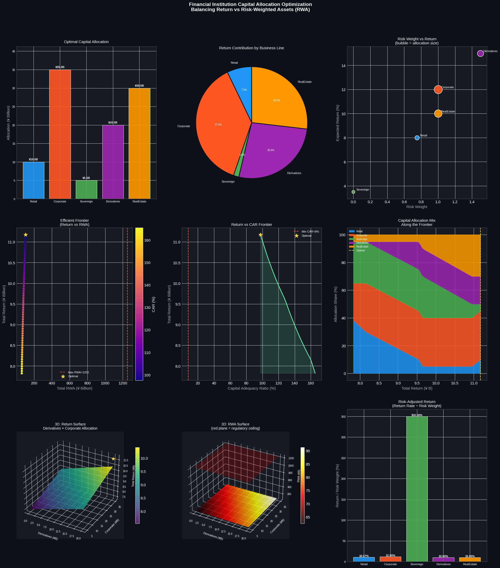
  Figure saved: capital_allocation.png

Key Takeaways

The model demonstrates three core insights that every bank treasurer should internalize:

1. RoRWA ≠ Optimal: Ranking solely by Return on RWA can be misleading when business lines have hard allocation bounds. The LP captures the full constraint interaction.

2. The Efficient Frontier is your negotiating tool: When presenting to regulators or the board, the frontier quantifies exactly what a change in the RWA ceiling is worth in euros of foregone return.

3. Shadow prices matter more than point solutions: The slope of the sensitivity curve (Chart E) — not just the optimal allocation — is what drives strategic capital planning conversations.