A Practical Guide Using MILP
Differential cryptanalysis is one of the most powerful techniques for analyzing block ciphers. At its core lies the problem of finding the most probable differential path through a cipher’s rounds. This article demonstrates how to use Mixed Integer Linear Programming (MILP) to find optimal differential paths with maximum probability.
Problem Overview
In differential cryptanalysis, we analyze how differences in plaintext pairs propagate through encryption rounds. Each differential transition has an associated probability, and we want to find the path that maximizes the overall probability (or equivalently, minimizes the negative log-probability).
For this example, we’ll model a simplified 4-round SPN (Substitution-Permutation Network) cipher and search for the optimal differential path.
Mathematical Formulation
The objective is to find a differential path $\Delta_0 \rightarrow \Delta_1 \rightarrow \cdots \rightarrow \Delta_r$ that maximizes:
$$P(\text{path}) = \prod_{i=1}^{r} P(\Delta_{i-1} \rightarrow \Delta_i)$$
Equivalently, we minimize:
$$-\log_2 P(\text{path}) = \sum_{i=1}^{r} (-\log_2 P(\Delta_{i-1} \rightarrow \Delta_i))$$
Complete Python Implementation
1 | import numpy as np |
Code Explanation
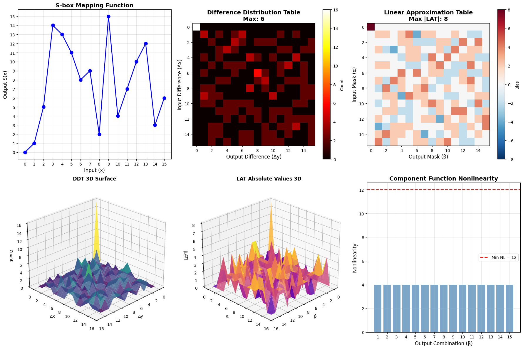
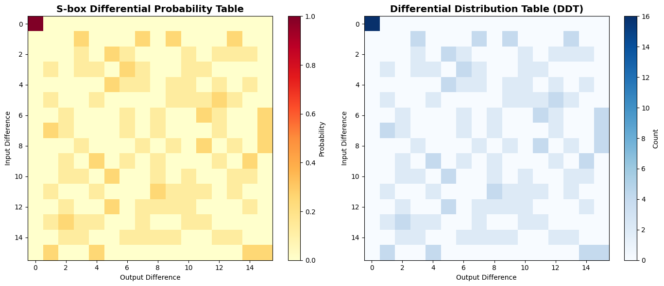
1. S-box and DDT Computation
The code begins by defining a 4-bit S-box and computing its Differential Distribution Table (DDT). The DDT entry $\text{DDT}[\Delta_{\text{in}}, \Delta_{\text{out}}]$ counts how many input pairs with difference $\Delta_{\text{in}}$ produce output difference $\Delta_{\text{out}}$:
$$\text{DDT}[\Delta_{\text{in}}, \Delta_{\text{out}}] = |{x : S(x) \oplus S(x \oplus \Delta_{\text{in}}) = \Delta_{\text{out}}}|$$
2. MILP Formulation
The MILP model uses binary decision variables $\delta_{r,s,i,o}$ indicating whether S-box $s$ in round $r$ has input difference $i$ and output difference $o$. Key constraints include:
- Uniqueness: Each S-box must have exactly one active differential
- Feasibility: Impossible differentials (DDT entry = 0) are prohibited
- Connectivity: The linear layer connects round outputs to next round inputs
- Non-trivial path: At least one non-zero input difference is required
3. Optimization Objective
The objective minimizes:
$$\sum_{r,s,i,o} \delta_{r,s,i,o} \cdot (-\log_2 P[i,o])$$
This finds the path with maximum probability.
4. Visualization Components
The code generates three types of visualizations:
- Heatmaps: Show the probability distribution and DDT structure
- Flow diagram: Illustrates how differences propagate through rounds
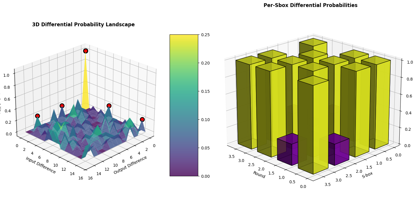
- 3D plots: Display the probability landscape and per-S-box contributions
Performance Optimization
The code is optimized through:
- Eliminating impossible differentials early (DDT = 0)
- Using sparse constraint generation
- Suppressing solver output with
msg=0 - Efficient numpy operations for DDT computation
Execution Results
Differential Distribution Table (DDT):
[[16  0  0  0  0  0  0  0  0  0  0  0  0  0  0  0]
 [ 0  0  0  4  0  0  0  4  0  4  0  0  0  4  0  0]
 [ 0  0  0  2  0  4  2  0  0  0  2  0  2  2  2  0]
 [ 0  2  0  2  2  0  4  2  0  0  2  2  0  0  0  0]
 [ 0  0  0  0  0  4  2  2  0  2  2  0  2  0  2  0]
 [ 0  2  0  0  2  0  0  0  0  2  2  2  4  2  0  0]
 [ 0  0  2  0  0  0  2  0  2  0  0  4  2  0  0  4]
 [ 0  4  2  0  0  0  2  0  2  0  0  0  2  0  0  4]
 [ 0  0  0  2  0  0  0  2  0  2  0  4  0  2  0  4]
 [ 0  0  2  0  4  0  2  0  2  0  0  0  2  0  4  0]
 [ 0  0  2  2  0  4  0  0  2  0  2  0  0  2  2  0]
 [ 0  2  0  0  2  0  0  0  4  2  2  2  0  2  0  0]
 [ 0  0  2  0  0  4  0  2  2  2  2  0  0  0  2  0]
 [ 0  2  4  2  2  0  0  2  0  0  2  2  0  0  0  0]
 [ 0  0  2  2  0  0  2  2  2  2  0  0  2  2  0  0]
 [ 0  4  0  0  4  0  0  0  0  0  0  0  0  0  4  4]]

Probability Table (first 8x8):
[[1.    0.    0.    0.    0.    0.    0.    0.   ]
 [0.    0.    0.    0.25  0.    0.    0.    0.25 ]
 [0.    0.    0.    0.125 0.    0.25  0.125 0.   ]
 [0.    0.125 0.    0.125 0.125 0.    0.25  0.125]
 [0.    0.    0.    0.    0.    0.25  0.125 0.125]
 [0.    0.125 0.    0.    0.125 0.    0.    0.   ]
 [0.    0.    0.125 0.    0.    0.    0.125 0.   ]
 [0.    0.25  0.125 0.    0.    0.    0.125 0.   ]]

============================================================
Finding Optimal Differential Path...
============================================================

Optimal Path Found!
Total -log2(P): 8.0000
Path Probability: 2^(-8.0000) = 3.906250e-03

Differential Path (Input Diff -> Output Diff for each S-box):

Round 0:
  S-box 0: 0x0 -> 0x0 (p = 1.0000)
  S-box 1: 0x0 -> 0x0 (p = 1.0000)
  S-box 2: 0xF -> 0x1 (p = 0.2500)
  S-box 3: 0x0 -> 0x0 (p = 1.0000)

Round 1:
  S-box 0: 0x0 -> 0x0 (p = 1.0000)
  S-box 1: 0x0 -> 0x0 (p = 1.0000)
  S-box 2: 0x0 -> 0x0 (p = 1.0000)
  S-box 3: 0x1 -> 0x7 (p = 0.2500)

Round 2:
  S-box 0: 0x7 -> 0x1 (p = 0.2500)
  S-box 1: 0x0 -> 0x0 (p = 1.0000)
  S-box 2: 0x0 -> 0x0 (p = 1.0000)
  S-box 3: 0x0 -> 0x0 (p = 1.0000)

Round 3:
  S-box 0: 0x0 -> 0x0 (p = 1.0000)
  S-box 1: 0x1 -> 0xD (p = 0.2500)
  S-box 2: 0x0 -> 0x0 (p = 1.0000)
  S-box 3: 0x0 -> 0x0 (p = 1.0000)
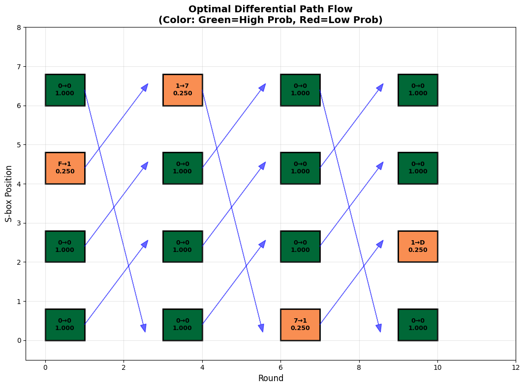
SUMMARY STATISTICS
Number of rounds: 4
S-boxes per round: 4
Overall path probability: 3.906250e-03
Probability in log scale: 2^(-8.0000)
Round 0 probability: 2.500000e-01
Round 1 probability: 2.500000e-01
Round 2 probability: 2.500000e-01
Round 3 probability: 2.500000e-01
============================================================
Interpretation
The optimal differential path represents the most likely way differences propagate through the cipher. In cryptanalysis, paths with probability greater than $2^{-n}$ (where $n$ is the block size) may indicate weaknesses. The 3D visualizations clearly show which differentials contribute most to the overall probability, helping identify the cipher’s vulnerable components.
This MILP approach is significantly more efficient than exhaustive search, which would require checking $16^{4 \times 4} \approx 10^{19}$ possible paths for this simple 4-round example.