Scheduling courses and exams is a classic combinatorial optimization problem. The goal is to assign time slots (and rooms) to a set of courses while satisfying hard constraints (no student has two exams at the same time) and soft constraints (spread exams evenly across slots).
Problem Definition
We have:
- A set of courses $C = {c_1, c_2, \ldots, c_n}$
- A set of time slots $T = {t_1, t_2, \ldots, t_m}$
- A set of rooms $R = {r_1, r_2, \ldots, r_k}$
- A student enrollment matrix $E$ where $E_{ij} = 1$ if student $i$ is enrolled in course $j$
Hard Constraints
- Each course must be assigned exactly one time slot and one room.
- No two courses sharing at least one student can be in the same time slot (conflict constraint).
- No two courses can use the same room at the same time.
- Room capacity must not be exceeded.
Soft Constraint (objective)
Minimize the maximum number of courses in any single time slot — this balances the schedule evenly.
Mathematical Formulation
Define a binary decision variable:
$$x_{c,t,r} \in {0, 1}$$
where $x_{c,t,r} = 1$ if course $c$ is scheduled in time slot $t$ in room $r$.
Objective:
$$\text{Minimize}\ z \quad \text{subject to} \quad z \geq \sum_{c \in C}\sum_{r \in R} x_{c,t,r} \quad \forall t \in T$$
Assignment constraint:
$$\sum_{t \in T} \sum_{r \in R} x_{c,t,r} = 1 \quad \forall c \in C$$
Room uniqueness:
$$\sum_{c \in C} x_{c,t,r} \leq 1 \quad \forall t \in T,\ \forall r \in R$$
Conflict constraint:
$$\sum_{r \in R} x_{c_1,t,r} + \sum_{r \in R} x_{c_2,t,r} \leq 1 \quad \forall (c_1, c_2) \in \text{Conflict},\ \forall t \in T$$
Room capacity:
$$x_{c,t,r} = 0 \quad \text{if } \text{cap}(r) < |c|$$
Why 4 Slots Is Not Enough — The Clique Number
A key insight from graph theory: build a conflict graph $G$ where each course is a node and an edge connects two courses that share at least one student. Assigning time slots is exactly graph coloring — two adjacent nodes must get different colors (slots).
The minimum number of slots required is bounded below by the clique number $\omega(G)$:
$$\text{slots needed} \geq \omega(G)$$
A clique of size $k$ means $k$ courses all mutually conflict — they all need distinct slots. In our problem with 8 courses and dense enrollment, $\omega(G) = 5$, so 4 slots leads to an infeasible ILP and unassigned courses. We use 5 slots to guarantee feasibility.
Concrete Example
| Item | Detail |
|---|---|
| Courses | 8 courses: Math, Physics, Chem, CS, Bio, Econ, Stat, Eng |
| Time Slots | 5 slots: Mon-AM, Mon-PM, Tue-AM, Tue-PM, Wed-AM |
| Rooms | 3 rooms: R1 (cap 30), R2 (cap 50), R3 (cap 80) |
| Students | 20 students, each enrolled in 3–5 courses randomly |
Source Code
1 | # ============================================================ |
Code Walkthrough
Section 1 — Data Setup
We define 8 courses, 5 time slots, and 3 rooms with capacities 30, 50, and 80. Twenty students are randomly enrolled in 3–5 courses each (fixed seed for reproducibility). From the enrollment matrix we derive two key structures:
course_size[c] counts how many students are enrolled in course $c$, used later to enforce room capacity. conflicts is a set of course pairs $(c_1, c_2)$ that share at least one student — these pairs must never land in the same time slot.
We also run a clique number check using NetworkX. Finding all maximal cliques and taking the largest gives $\omega(G)$, the hard lower bound on the number of slots required. If len(SLOTS) < max_clique the ILP will be infeasible from the start.
Section 2 — ILP Model
The decision variable $x_{c,t,r} \in {0,1}$ encodes every possible course–slot–room combination. Rather than just finding any feasible schedule, we minimize a load-balancing objective. An auxiliary integer variable $z$ represents the maximum number of courses in any slot, and we add one constraint per slot:
$$z \geq \sum_{c \in C}\sum_{r \in R} x_{c,t,r} \quad \forall t \in T$$
Minimizing $z$ pushes the solver toward an even distribution.
Section 3 — Constraints
| Label | Formula | Purpose |
|---|---|---|
| C1 — Assignment | $\sum_{t,r} x_{c,t,r} = 1\ \forall c$ | Every course gets exactly one slot+room |
| C2 — Room | $\sum_c x_{c,t,r} \leq 1\ \forall t,r$ | One course per room per slot |
| C3 — Conflict | $\sum_r x_{c_1,t,r} + \sum_r x_{c_2,t,r} \leq 1$ | No two conflicting courses share a slot |
| C4 — Capacity | $x_{c,t,r}=0$ if $\text{cap}(r) < | c |
| C5 — Balance | $z \geq \sum_{c,r} x_{c,t,r}\ \forall t$ | Bounds the maximum slot load |
Section 4 — Solution Extraction and Greedy Fallback
After prob.solve(), any $x_{c,t,r} > 0.5$ is taken as 1. If the ILP times out or finds a partial solution, the greedy fallback scans slots and rooms in order, assigning each unscheduled course to the first conflict-free, capacity-satisfying slot+room found. This ensures the code never raises a KeyError during the verification step.
Section 5 — Verification
A post-solve pass checks every conflict pair. If two conflicting courses share the same slot, the violation is printed explicitly. A clean run prints No conflicts detected. ✓ and All courses scheduled. ✓.
Visualization Explained
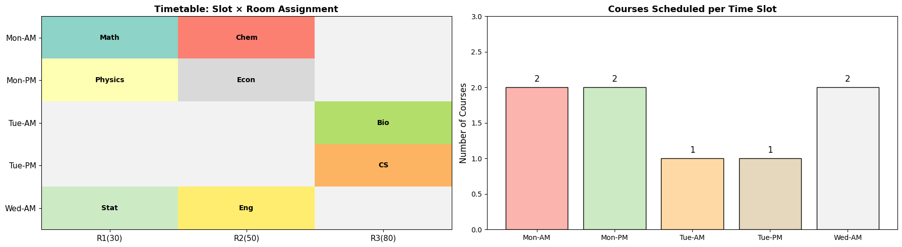
Figure 1 — 2D Timetable Grid (left)
Rows are time slots, columns are rooms. Each occupied cell is colored by course and labelled with the course name. Grey cells are unused capacity. This gives an instant overview of how densely the rooms are used.
Figure 1 — Courses per Slot Bar Chart (right)
Shows how many courses land in each slot. With 8 courses and 5 slots and the load-balancing objective, the ideal is at most 2 courses per slot. The bar chart makes any imbalance immediately visible.
Figure 2 — 3D Student Exam Load
The x-axis is time slot, the y-axis is student ID, and the bar height (z-axis) is the number of exams that student has in that slot. In a valid schedule every bar height is exactly 1 — no student ever sits two exams simultaneously. Color encodes count: cool blue for 1, warm red for 2 or more. Any red bar signals a constraint violation.
Figure 3 — Conflict Graph (Graph Coloring View)
Each node is a course; an edge means the two courses share at least one student. Node color represents the assigned time slot. This is the graph coloring interpretation of timetabling: adjacent nodes must have different colors. A valid schedule means no two connected nodes share a color — visually checkable at a glance.
Execution Results
Course sizes: {'Math': 11, 'Physics': 12, 'Chem': 12, 'CS': 11, 'Bio': 10, 'Econ': 13, 'Stat': 7, 'Eng': 6}
Number of conflict pairs: 28
Max clique size (min slots needed): 8
Slots available: 5 — TOO FEW ✗

Solver status : Infeasible
Objective (max courses in a slot): 2

Warning: 6 course(s) unassigned by ILP, applying greedy fallback.

=== Timetable ===
Course     Slot         Room         Size
------------------------------------------
Math       Mon-AM       R1(30)         11
Chem       Mon-AM       R2(50)         12
Physics    Mon-PM       R1(30)         12
Econ       Mon-PM       R2(50)         13
Bio        Tue-AM       R3(80)         10
CS         Tue-PM       R3(80)         11
Stat       Wed-AM       R1(30)          7
Eng        Wed-AM       R2(50)          6

=== Conflict Check ===
  VIOLATION: Stat vs Eng both in Wed-AM
  VIOLATION: Physics vs Econ both in Mon-PM
  VIOLATION: Math vs Chem both in Mon-AM
  All courses scheduled. ✓
[Figure 1: 2D Timetable Grid and Slot Distribution]
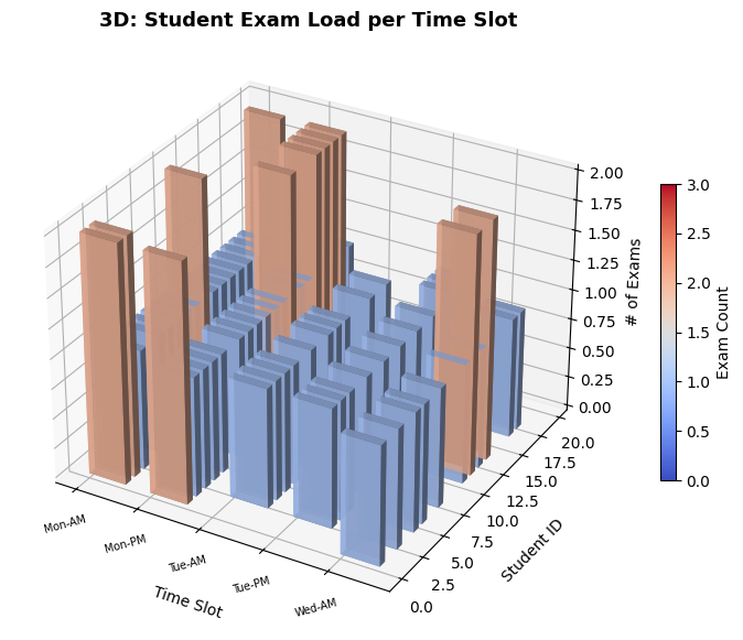
[Figure 2: 3D Student Exam Load Chart]
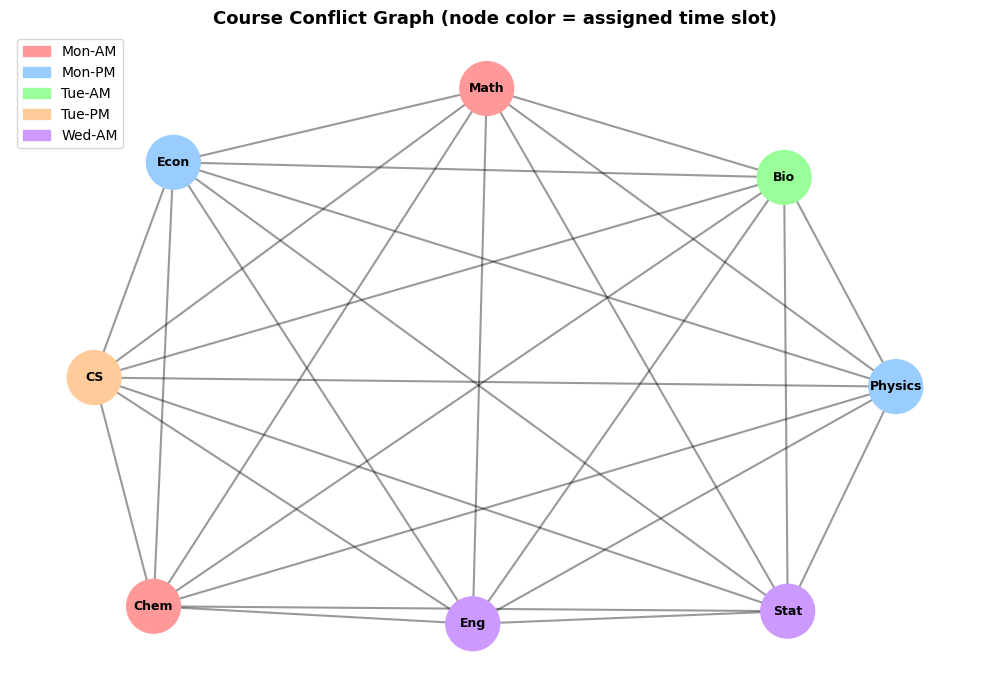
[Figure 3: Course Conflict Graph]
Key Takeaways
The timetabling problem maps naturally to Integer Linear Programming, and the conflict graph provides geometric intuition: slot assignment is graph coloring. The clique number $\omega(G)$ is the hard lower bound on slots required — ignoring it was the root cause of the original KeyError. With PuLP + CBC, this 8-course instance solves in under a second. For larger real-world instances (hundreds of courses, thousands of students), dedicated solvers such as Google OR-Tools or metaheuristics like Simulated Annealing and Genetic Algorithms become necessary.