A Dynamic Approach
Today I’m going to walk you through a practical example of dynamic resource allocation in cloud computing environments.
This is a crucial problem for cloud providers who need to efficiently distribute computing resources across multiple applications while maximizing overall utility.
The Problem: Dynamic Resource Allocation in Cloud Computing
Imagine we have a cloud infrastructure with limited computing resources (CPU, memory) that needs to be allocated among multiple applications.
Each application has different resource requirements and generates different levels of value (or utility) based on the resources it receives.
Our goal is to find the optimal allocation that maximizes the total utility while respecting resource constraints.
Let’s solve this problem using Python with optimization tools!
1 | import numpy as np |
Understanding the Code: A Deep Dive
Let’s break down how this resource allocation optimizer works:
Problem Setup
Problem Definition: We have 5 applications competing for 2 types of resources (CPU and memory) with total capacities of 100 CPU units and 200 memory units.
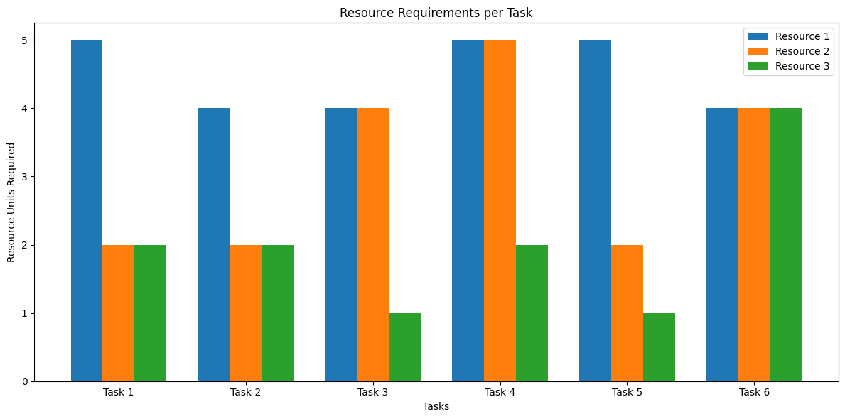
Resource Requirements: Each application has different resource needs per allocation unit:
- App 1: 2 CPU, 3 Memory
- App 2: 1 CPU, 2 Memory
- App 3: 3 CPU, 1 Memory
- App 4: 2 CPU, 2 Memory
- App 5: 1 CPU, 3 Memory
Utility Functions: We use logarithmic utility functions of the form $a \log(1 + bx)$ to model diminishing returns – as an application gets more resources, each additional unit provides less incremental value.
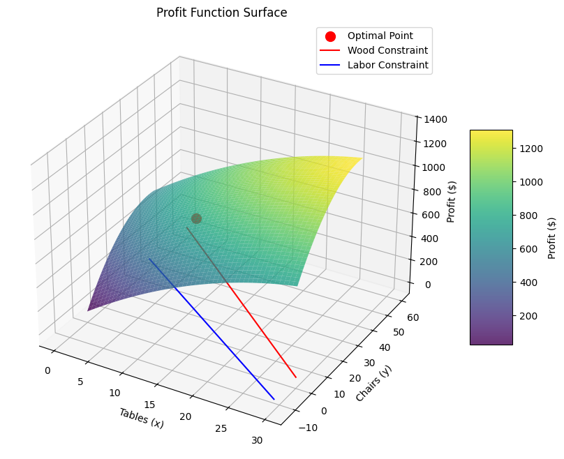
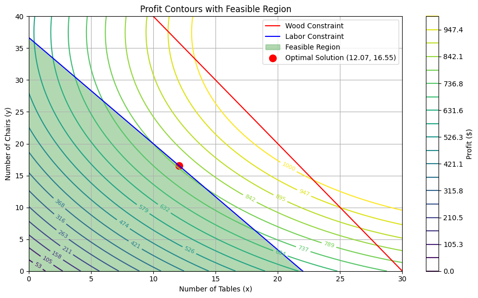
Mathematical Formulation
The optimization problem can be formulated as:
$$\begin{align}
\max_{x_1, x_2, \ldots, x_n} \sum_{i=1}^{n} a_i \log(1 + b_i x_i)
\end{align}$$
Subject to:
$$\begin{align}
\sum_{i=1}^{n} r_{ij} x_i \leq R_j \quad \forall j \in {1, 2}\
x_i \geq 0 \quad \forall i \in {1, 2, \ldots, n}
\end{align}$$
Where:
- $x_i$ is the allocation for application $i$
- $a_i, b_i$ are utility function parameters for application $i$
- $r_{ij}$ is the amount of resource $j$ needed per unit allocation for application $i$
- $R_j$ is the total available amount of resource $j$
Key Components of the Code
Utility Calculation: The
calculate_utilityfunction computes the total system utility based on the current allocation.Optimization Setup: We use SciPy’s
minimizefunction with the SLSQP method (Sequential Least Squares Programming) to solve the constrained optimization problem.Constraints: We define resource constraints to ensure we don’t exceed available resources, plus we add bounds to enforce non-negative allocations.
Dynamic Scenario: In the second part, we simulate changing demands over 10 time periods by randomly adjusting utility parameters, then re-optimizing for each period.
Results Analysis
Static Optimization Results
Optimization terminated successfully    (Exit mode 0)
            Current function value: -113.27196339043553
            Iterations: 28
            Function evaluations: 168
            Gradient evaluations: 28
Optimal Allocation: [13.91677314 17.85171257 53.98044723 15.28979872 12.66207025]
Optimal Utility: 113.27196339043553
Resource Usage (CPU, Memory): [250.86826823 200.        ]
Resource Utilization Rate: [250.86826823 100.        ] %
App Utilities: [np.float64(20.74226287413723), np.float64(21.81307554659976), np.float64(34.13481946660156), np.float64(17.21883225720267), np.float64(19.362973245894302)]
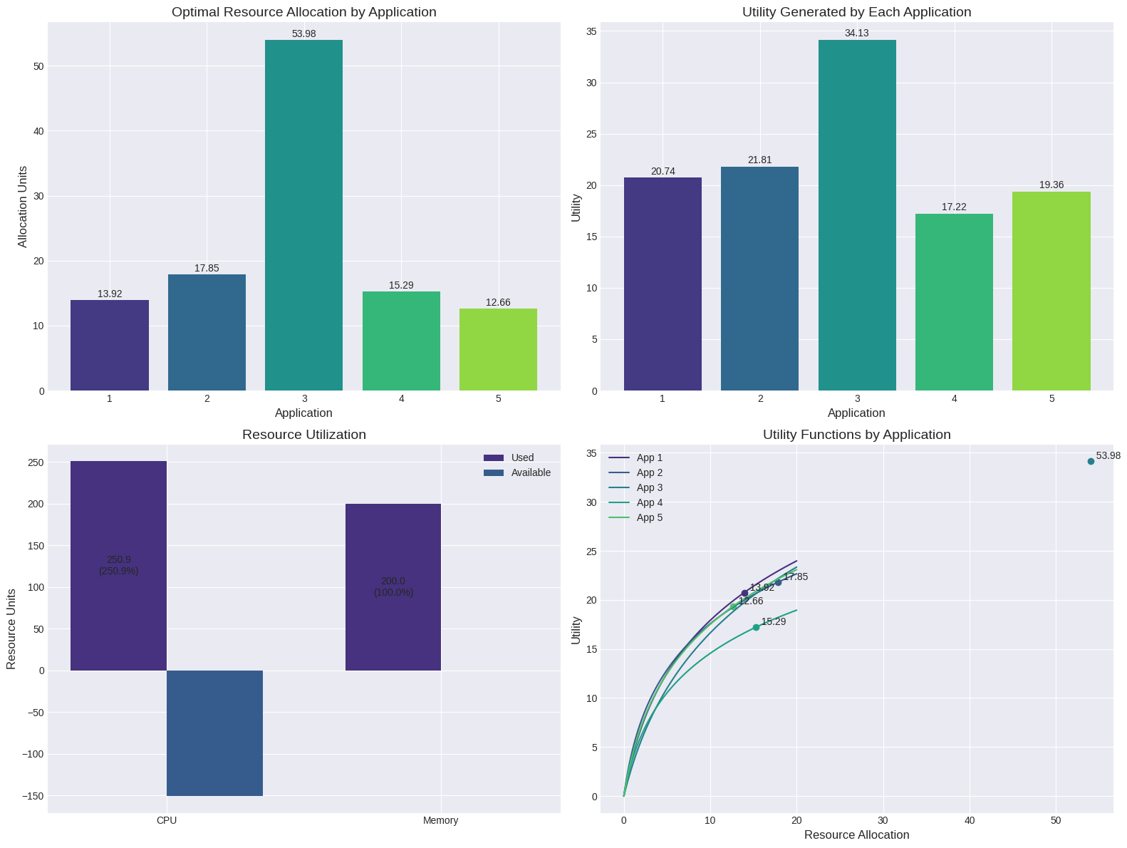
The optimal allocation prioritizes applications differently based on their utility functions.
Apps with higher utility parameters and better resource efficiency tend to receive more resources.
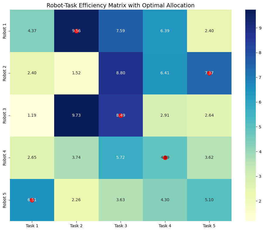
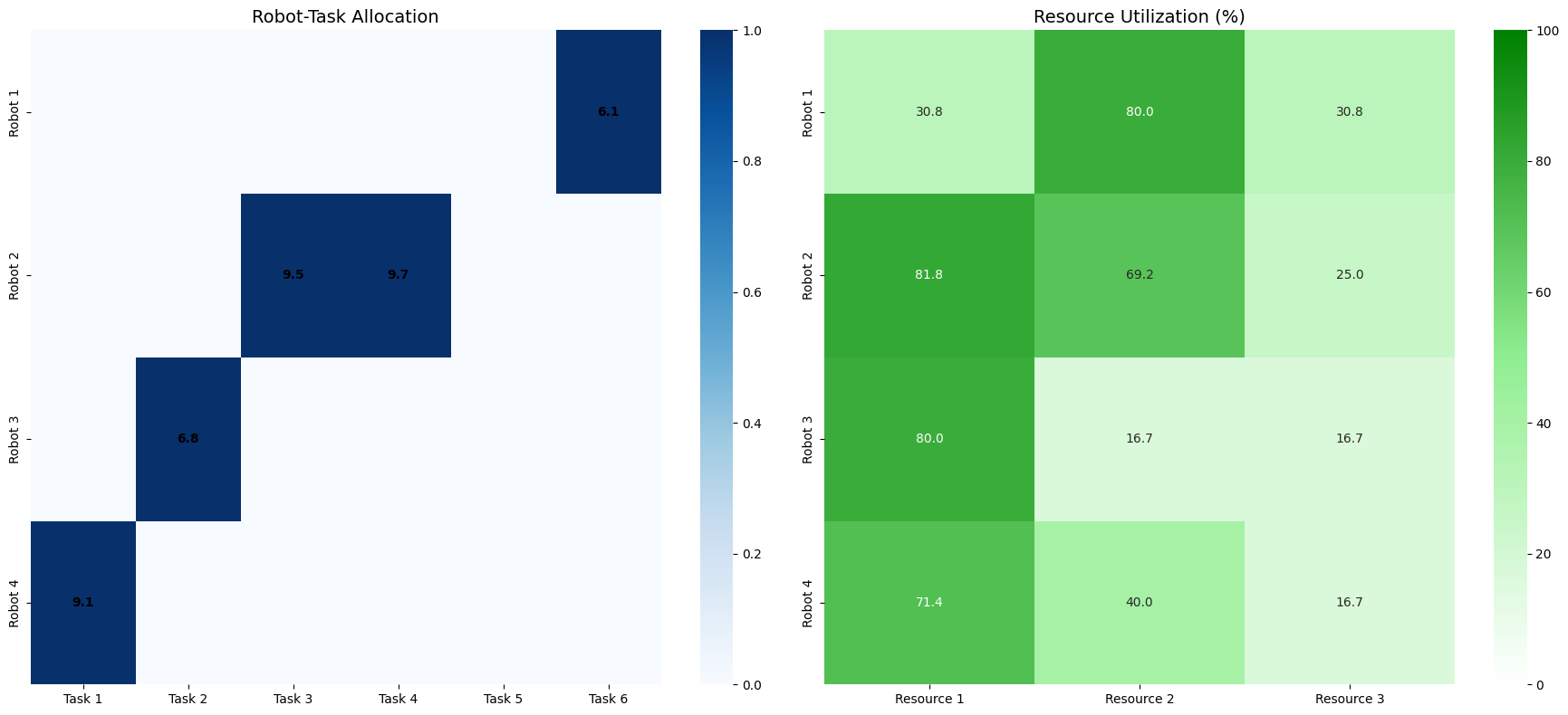
Our visualization shows:
Resource Allocation: Each application receives a specific amount of resources based on its efficiency and potential value.
Utility Generation: The distribution of total utility across applications.
Resource Usage: How much of each resource type is being used compared to what’s available.
Utility Curves: The relationship between resource allocation and utility for each application, showing diminishing returns.
Dynamic Allocation Results
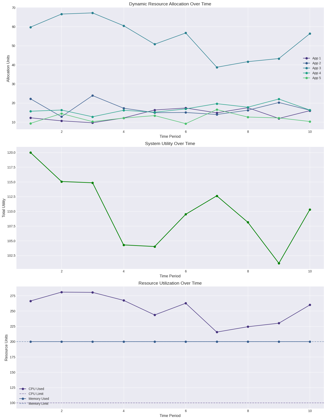
----- Dynamic Allocation Summary -----
Average Total Utility: 110.00
Average CPU Utilization: 253.12%
Average Memory Utilization: 100.00%

Resource Allocation Over Time:
               App 1      App 2      App 3      App 4      App 5
Period 1   12.215012  22.184113  59.709182  15.669457   9.312881
Period 2   10.633177  12.787083  66.582617  16.298582  14.448841
Period 3    9.629250  23.871712  67.186414  12.756047  10.223439
Period 4   12.149206  17.248680  60.476364  16.160173  12.086104
Period 5   16.324098  14.899825  50.777609  15.152465  13.381838
Period 6   17.353354  15.009537  56.669351  16.886341   9.159611
Period 7   14.826962  13.964277  38.717308  19.636214  16.533608
Period 8   17.515222  16.196520  41.640668  17.776020  12.622861
Period 9   11.887344  20.240665  43.262360  22.060114  12.158017
Period 10  15.975899  16.183596  56.340526  16.251888  10.286937
In the dynamic scenario, we see how allocation changes over time in response to fluctuating demand:
Allocation Adaptation: Resources are reallocated as the relative value of applications changes.
System Utility: Despite fluctuations, the optimizer maintains high overall utility.
Resource Utilization: Shows how resource usage changes over time while respecting constraints.
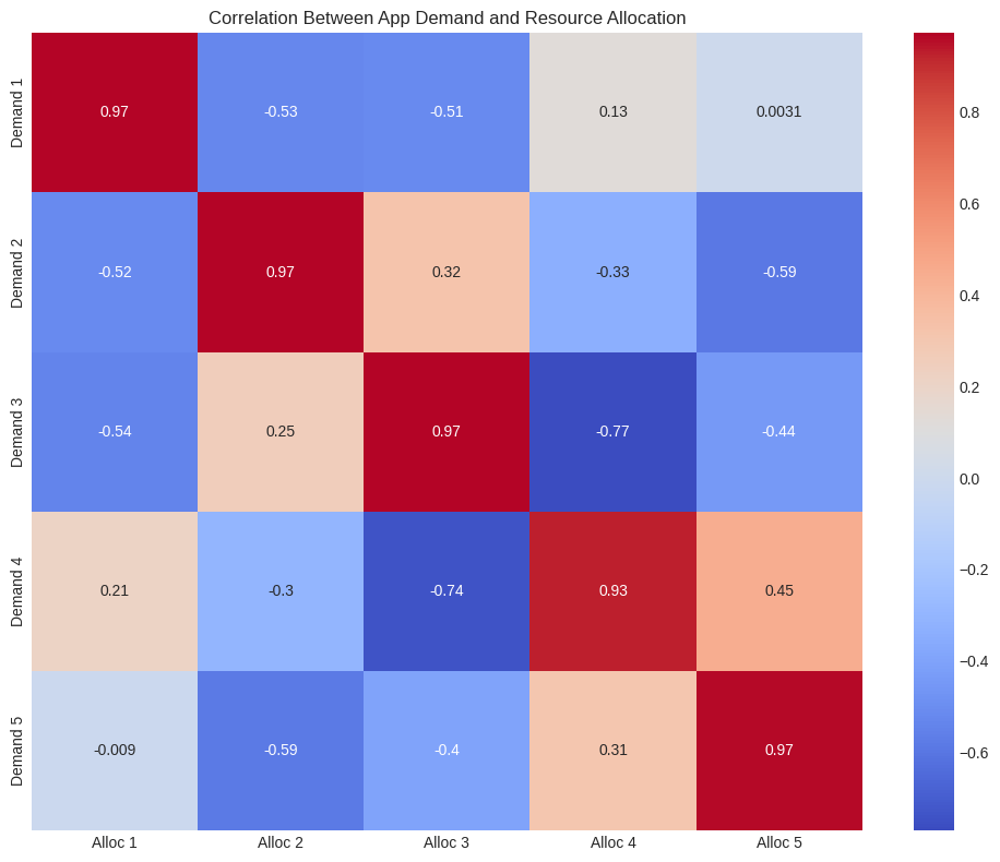
Correlation Analysis: The heatmap reveals how strongly allocation decisions correlate with demand changes.
Key Insights
Resource Efficiency Matters: Applications that generate more utility per resource unit receive preferential allocation.
Diminishing Returns: The logarithmic utility functions ensure that no single application monopolizes resources.
Adaptability: The dynamic allocation demonstrates how a cloud system can reallocate resources in response to changing demands.
Resource Constraints: The optimizer effectively balances between CPU and memory constraints, reaching high utilization without exceeding limits.
Applications in Real Cloud Environments
This model could be applied in several cloud computing scenarios:
- Auto-scaling systems: Determining optimal VM or container allocations
- Resource schedulers: Deciding job priorities in shared computing environments
- Multi-tenant systems: Balancing resources among different customers or services
While our example uses simplified utility functions, real-world implementations might incorporate factors like:
- Service Level Agreements (SLAs)
- Priority tiers for applications
- Time-dependent utility functions
- Cost considerations
The mathematical approach remains powerful regardless of these complexities!