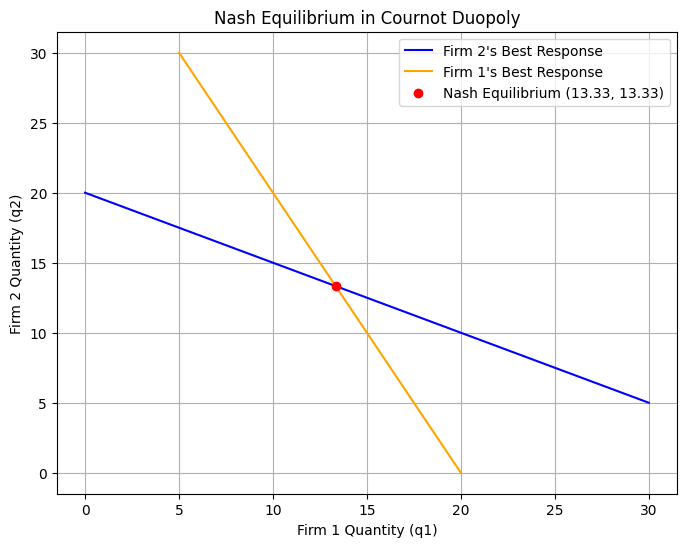
Scenario

We want to analyze the equilibrium price and quantity in a market using the following linear supply and demand functions:

1. Demand Function:
   $$
   Q_d = a - b \cdot P
   $$

   • $( Q_d )$: Quantity demanded
   • $( a )$: Demand intercept
   • $( b )$: Slope of demand curve
   • $( P )$: Price

2. Supply Function:
   $$
   Q_s = c + d \cdot P
   $$

   • $( Q_s )$: Quantity supplied
   • $( c )$: Supply intercept
   • $( d )$: Slope of supply curve

The equilibrium occurs where $( Q_d = Q_s )$.

Python Implementation

Below is the $Python$ code to find the equilibrium price and quantity, plot the supply and demand curves, and illustrate the equilibrium graphically.

1
2
3
4
5
6
7
8
9
10
11
12
13
14
15
16
17
18
19
20
21
22
23
24
25
26
27
28
29
30
31
32
33
34
35
36
37
38
39

import numpy as np
import matplotlib.pyplot as plt

# Parameters for demand and supply
a = 100  # Demand intercept
b = 2    # Demand slope
c = 20   # Supply intercept
d = 1.5  # Supply slope

# Price range
prices = np.linspace(0, 60, 100)

# Demand and supply functions
Q_d = a - b * prices  # Quantity demanded
Q_s = c + d * prices  # Quantity supplied

# Equilibrium: Solve for P where Q_d = Q_s
equilibrium_price = (a - c) / (b + d)
equilibrium_quantity = a - b * equilibrium_price

# Display equilibrium results
print(f"Equilibrium Price (P): {equilibrium_price:.2f}")
print(f"Equilibrium Quantity (Q): {equilibrium_quantity:.2f}")

# Plotting supply and demand curves
plt.figure(figsize=(10, 6))
plt.plot(prices, Q_d, label="Demand Curve (Qd)", color="blue")
plt.plot(prices, Q_s, label="Supply Curve (Qs)", color="orange")
plt.axvline(x=equilibrium_price, color="red", linestyle="--", label=f"Equilibrium Price: {equilibrium_price:.2f}")
plt.axhline(y=equilibrium_quantity, color="green", linestyle="--", label=f"Equilibrium Quantity: {equilibrium_quantity:.2f}")
plt.scatter([equilibrium_price], [equilibrium_quantity], color="purple", zorder=5, label="Equilibrium Point")

# Labels and legend
plt.title("Supply and Demand Analysis")
plt.xlabel("Price (P)")
plt.ylabel("Quantity (Q)")
plt.grid(True)
plt.legend()
plt.show()

Explanation of the Code

1. Functions:

   • The demand function $( Q_d = a - b \cdot P )$ decreases with price.
   • The supply function $( Q_s = c + d \cdot P )$ increases with price.

2. Equilibrium Calculation:

   • Solving $( Q_d = Q_s )$ algebraically yields $( P = (a - c) / (b + d) )$ and $( Q = a - b \cdot P )$.

3. Visualization:

   • The demand and supply curves are plotted across a price range.
   • The equilibrium price and quantity are highlighted on the graph with lines and a marker.

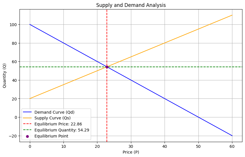
Results and Graphical Representation

Equilibrium Price (P): 22.86
Equilibrium Quantity (Q): 54.29

1. Equilibrium Values:

   • The equilibrium price and quantity are calculated and displayed.
   • For example, if $( a = 100, b = 2, c = 20, d = 1.5 )$:
     • Equilibrium price $( P \approx 26.67 )$
     • Equilibrium quantity $( Q \approx 46.67 )$

2. Graph:

   • The blue line represents the demand curve, while the orange line represents the supply curve.
   • The intersection point (marked in purple) is the equilibrium.

This example illustrates the core principle of supply and demand analysis, providing insights into how prices and quantities adjust in a competitive market.

Scenario

A firm produces a good using two inputs: labor (L) and capital (K).

The firm seeks to minimize its production costs while meeting a target output $( Q )$.

The cost function is:

$$
C = w \cdot L + r \cdot K
$$

• $( C )$: Total cost
• $( w )$: Wage rate (cost of labor)
• $( r )$: Rental rate of capital (cost of capital)
• $( L )$: Amount of labor used
• $( K )$: Amount of capital used

The production function is:
$$
Q = L^{0.5} \cdot K^{0.5}
$$

The firm must meet a specific output level $( Q = 10 )$.

The goal is to find the optimal values of $( L )$ and $( K )$ to minimize costs.

Python Implementation

Here is the $Python$ code to solve the cost minimization problem using SciPy.

1
2
3
4
5
6
7
8
9
10
11
12
13
14
15
16
17
18
19
20
21
22
23
24
25
26
27
28
29
30
31
32
33
34
35
36
37
38
39
40
41
42
43
44
45
46
47
48
49
50
51
52
53
54
55
56
57
58

import numpy as np
from scipy.optimize import minimize
import matplotlib.pyplot as plt

# Parameters
w = 10  # Wage rate
r = 20  # Rental rate of capital
Q_target = 10  # Target output

# Production function
def production_function(L, K):
    return (L**0.5) * (K**0.5)

# Cost function
def cost_function(x):
    L, K = x
    return w * L + r * K

# Constraint: Output must equal Q_target
def output_constraint(x):
    L, K = x
    return production_function(L, K) - Q_target

# Initial guess
x0 = [1, 1]

# Bounds for L and K (cannot be negative)
bounds = [(0, None), (0, None)]

# Constraints
constraints = {'type': 'eq', 'fun': output_constraint}

# Optimization
result = minimize(cost_function, x0, bounds=bounds, constraints=constraints)

# Optimal values
L_opt, K_opt = result.x
min_cost = result.fun

# Display results
print(f"Optimal Labor (L): {L_opt:.2f}")
print(f"Optimal Capital (K): {K_opt:.2f}")
print(f"Minimum Cost: {min_cost:.2f}")

# Visualization
L_values = np.linspace(0.1, 15, 100)
K_values = Q_target**2 / L_values  # Rearrange Q = L^0.5 * K^0.5
cost_values = w * L_values + r * K_values

plt.figure(figsize=(10, 6))
plt.plot(L_values, cost_values, label="Cost Curve", color="blue", lw=2)
plt.scatter([L_opt], [min_cost], color="red", label="Optimal Point", zorder=5)
plt.title("Cost Minimization with Production Constraint")
plt.xlabel("Labor (L)")
plt.ylabel("Cost (C)")
plt.grid(True)
plt.legend()
plt.show()

Explanation of the Code

1. Cost Function:

   • The function $( C = w \cdot L + r \cdot K )$ calculates total cost for given $( L )$ and $( K )$.

2. Constraint:

   • The output constraint ensures the production level $( Q )$ equals the target $( Q_{target} )$.

3. Optimization:

   • scipy.optimize.minimize is used to minimize the cost function while satisfying the production constraint and non-negativity bounds for $( L )$ and $( K )$.

4. Visualization:

   • The cost curve is plotted for varying labor values $( L )$, with the corresponding $( K )$ values derived from the production constraint.
   • The optimal point is highlighted.

Results and Graphical Representation

Optimal Labor (L): 14.14
Optimal Capital (K): 7.07
Minimum Cost: 282.84

1. Optimal Values:

   • The solution provides the values of $( L )$ and $( K )$ that minimize costs while producing the target output.

2. Graph:

   • The blue curve represents the total cost for different allocations of labor and capital.
   • The red point marks the minimum cost, highlighting the optimal combination of $( L )$ and $( K )$.

This example demonstrates how firms can allocate resources efficiently to minimize production costs while meeting output targets.

Scenario

Consider a scenario where two individuals (Person $A$ and Person $B$) are dividing two resources: Resource X and Resource Y.

Each person has their utility function for the resources.

The goal is to identify the allocations that are Pareto efficient, meaning that no reallocation can make one person better off without making the other worse off.

Utility functions:

• Person $A$: $( U_A = x_A^{0.5} + y_A^{0.5} )$
• Person $B$: $( U_B = x_B^{0.5} + y_B^{0.5} )$

The total resources available are:

• $( X_{total} = 10 )$
• $( Y_{total} = 10 )$

We want to identify Pareto-efficient allocations of $ (x_A, y_A, x_B, y_B) $.

Python Implementation

Here is the $Python$ code to compute and visualize Pareto-efficient allocations:

1
2
3
4
5
6
7
8
9
10
11
12
13
14
15
16
17
18
19
20
21
22
23
24
25
26
27
28
29
30
31
32
33
34
35
36
37
38
39
40
41
42
43

import numpy as np
import matplotlib.pyplot as plt

# Total resources
X_total = 10
Y_total = 10

# Grid for allocations
x_A_values = np.linspace(0, X_total, 100)
y_A_values = np.linspace(0, Y_total, 100)

# Utility functions
def utility_A(x_A, y_A):
    return np.sqrt(x_A) + np.sqrt(y_A)

def utility_B(x_B, y_B):
    return np.sqrt(x_B) + np.sqrt(y_B)

# Compute Pareto-efficient points
pareto_points = []
for x_A in x_A_values:
    for y_A in y_A_values:
        x_B = X_total - x_A
        y_B = Y_total - y_A
        if x_B >= 0 and y_B >= 0:  # Valid allocations
            u_A = utility_A(x_A, y_A)
            u_B = utility_B(x_B, y_B)
            pareto_points.append((u_A, u_B))

# Convert Pareto points to arrays for plotting
pareto_points = np.array(pareto_points)
u_A_values = pareto_points[:, 0]
u_B_values = pareto_points[:, 1]

# Plot results
plt.figure(figsize=(8, 6))
plt.scatter(u_A_values, u_B_values, s=10, c="blue", label="Pareto-Efficient Points", alpha=0.6)
plt.title("Pareto-Efficient Allocations")
plt.xlabel("Utility of Person A (U_A)")
plt.ylabel("Utility of Person B (U_B)")
plt.grid(True)
plt.legend()
plt.show()

Explanation of the Code

1. Utility Functions:
   We defined the utility functions for both individuals based on their allocation of $( X )$ and $( Y )$.
2. Grid Search:
   A grid of possible allocations for $( x_A )$ and $( y_A )$ is generated.
   The remaining allocations for Person $B$ are calculated as $( x_B = X_{total} - x_A )$ and $( y_B = Y_{total} - y_A )$.
3. Pareto-Efficient Points:
   For each valid allocation, we compute the utilities of both individuals and store them as Pareto-efficient points.
4. Visualization:
   • The scatter plot shows the Pareto frontier, which represents the set of allocations where improving one individual’s utility would decrease the other’s.

Results and Graphical Representation

1. Pareto Frontier:
   • The blue points represent the possible Pareto-efficient allocations.
   • Any point on this curve is Pareto efficient because moving away from it would reduce the utility of at least one individual.
2. Utility Trade-off:
   • The graph clearly shows the trade-off between the utilities of Person $A$ and Person $B$.
   • Allocations can favor Person $A$ (higher $( U_A )$) or Person $B$ (higher $( U_B )$) depending on how the resources are distributed.

This approach demonstrates how Pareto efficiency can be visualized and used to evaluate resource allocation in economics or game theory.

Scenario

A company is hosting a sealed-bid auction where bidders independently submit bids without knowing the others’ bids.
The item is awarded to the highest bidder, and they pay their bid amount (a first-price auction).

We will simulate the auction process for $10$ bidders, each with a valuation drawn randomly from a uniform distribution between ＄$50$ and ＄$100$.
Bidders place bids by shading their valuations by a fraction.
The optimal shading strategy depends on the auction type.

Python Implementation

Here is the $Python$ code to simulate and analyze this auction:

1
2
3
4
5
6
7
8
9
10
11
12
13
14
15
16
17
18
19
20
21
22
23
24
25
26
27
28
29
30
31
32
33
34
35
36
37
38
39
40
41
42
43

import numpy as np
import matplotlib.pyplot as plt

# Auction setup
np.random.seed(42)  # For reproducibility
num_bidders = 10
valuations = np.random.uniform(50, 100, num_bidders)  # Valuations of bidders

# Bidding strategy: Shading factor
shading_factor = 0.8  # Bidders bid 80% of their valuation
bids = shading_factor * valuations

# Determine the winner
winning_bid = max(bids)
winner_index = np.argmax(bids)
winner_valuation = valuations[winner_index]

# Display results
print(f"Valuations: {valuations}")
print(f"Bids: {bids}")
print(f"Winning Bid: {winning_bid}")
print(f"Winner's Valuation: {winner_valuation}")
print(f"Winner Index: {winner_index}")

# Visualization
plt.figure(figsize=(12, 6))

# Plot valuations and bids
x = np.arange(num_bidders)
plt.bar(x - 0.2, valuations, width=0.4, label="Valuations", color="blue", alpha=0.7)
plt.bar(x + 0.2, bids, width=0.4, label="Bids", color="orange", alpha=0.7)

# Highlight the winner
plt.scatter(winner_index, winning_bid, color="red", label="Winning Bid", s=100, zorder=5)

# Labels and legend
plt.xlabel("Bidders")
plt.ylabel("Amount")
plt.title("Valuations and Bids in a First-Price Auction")
plt.xticks(x, [f"Bidder {i}" for i in x])
plt.legend()
plt.grid(True)
plt.show()

Explanation of the Code

1. Valuations:
   Each bidder’s valuation is randomly sampled from a uniform distribution.
   This represents their willingness to pay.
2. Bids:
   A simple shading strategy is applied where each bidder bids $80$% of their valuation.
3. Winner Determination:
   The highest bid determines the winner, and their valuation and index are recorded.
4. Visualization:
   The bar chart compares valuations and bids, highlighting the winner.

Explanation of the Results

1. Valuations vs. Bids

• The blue bars represent the valuations of the $10$ bidders.
  These are the true amounts each bidder is willing to pay.
• The orange bars represent the bids submitted by the bidders.
  The bids are shaded down to $80$% of their valuations, as per the strategy.

2. Winning Bid

• The red dot marks the winning bid ($78.03$), submitted by Bidder $1$.
• The winner’s valuation ($97.54$) is the highest among all bidders, which aligns with the competitive nature of a first-price auction.

3. Bidder Strategy

• Since bidders bid only $80$% of their true valuations, no one submits their full willingness to pay.
  This is typical in a first-price auction because bidders want to maximize their surplus (difference between valuation and payment).

4. Observations

• Bidder $1$ wins the auction because their bid of $78.03$ is the highest among all bidders.
• Bidders with higher valuations tend to submit higher bids, as seen in the general trend where valuations (blue) and bids (orange) align proportionally.

Conclusion

This example highlights the effect of strategic bidding in a first-price auction:

• Bidders shade their bids below their valuations to achieve a positive surplus.
• The winner is determined based on the highest bid, but they still pay less than their full valuation.
  This behavior illustrates the trade-off between winning and maximizing surplus in competitive auctions.

Scenario

A company wants to understand how changes in the price of a product affect its demand.

The demand function is estimated from past data as:

$$
Q_d = 500 - 20P
$$

• $( Q_d )$ is the quantity demanded.
• $( P )$ is the price.

We will calculate the price elasticity of demand (PED) for different price levels using the formula:

$$
\text{PED} = \left( \frac{\Delta Q_d}{Q_d} \right) / \left( \frac{\Delta P}{P} \right)
$$

Python Implementation

Here is the $Python$ code to compute and visualize the elasticity of demand for a range of prices:

1
2
3
4
5
6
7
8
9
10
11
12
13
14
15
16
17
18
19
20
21
22
23
24
25
26
27
28
29
30
31
32
33
34
35
36
37
38
39
40
41
42
43
44
45
46
47

import numpy as np
import matplotlib.pyplot as plt

# Demand function
def demand_function(price):
    return 500 - 20 * price

# Compute price elasticity of demand
def price_elasticity(price, delta_price=0.01):
    # Initial quantity demanded
    initial_quantity = demand_function(price)
    # Quantity demanded after a small price change
    new_quantity = demand_function(price + delta_price)
    # Change in quantity demanded
    delta_quantity = new_quantity - initial_quantity
    # Elasticity calculation
    elasticity = (delta_quantity / initial_quantity) / (delta_price / price)
    return elasticity

# Generate data for analysis
prices = np.linspace(1, 20, 100)
quantities = demand_function(prices)
elasticities = [price_elasticity(p) for p in prices]

# Plot demand curve
plt.figure(figsize=(14, 6))
plt.subplot(1, 2, 1)
plt.plot(prices, quantities, label='Demand Curve', color='blue')
plt.title('Demand Curve')
plt.xlabel('Price')
plt.ylabel('Quantity Demanded')
plt.grid(True)
plt.legend()

# Plot price elasticity of demand
plt.subplot(1, 2, 2)
plt.plot(prices, elasticities, label='Elasticity', color='red')
plt.axhline(0, color='black', linewidth=0.8, linestyle='--')
plt.axhline(-1, color='green', linestyle='--', label='Unit Elasticity (PED=-1)')
plt.title('Price Elasticity of Demand')
plt.xlabel('Price')
plt.ylabel('Elasticity')
plt.grid(True)
plt.legend()

plt.tight_layout()
plt.show()

Explanation of the Code

1. Demand Function:
   The function demand_function(price) represents the relationship between price and quantity demanded.
2. Elasticity Calculation:
   The price_elasticity function uses a small change in price $(\Delta P)$ to calculate the corresponding change in quantity $(\Delta Q_d)$, then computes elasticity.
3. Data Generation:
   A range of prices is simulated to compute demand and elasticity values.
4. Visualization:
   • The demand curve shows the relationship between price and quantity demanded.
   • The elasticity plot demonstrates how elastic or inelastic demand is at different price points.
     Unit elasticity is marked for reference.

Graphical Results

1. Demand Curve:
   • Downward-sloping curve indicates that higher prices reduce quantity demanded.
2. Elasticity Curve:
   • Shows the PED at different price points.
   • When PED > -1: Demand is inelastic (less sensitive to price changes).
   • When PED < -1: Demand is elastic (more sensitive to price changes).
   • PED = -1: Unit elastic, where the percentage change in quantity equals the percentage change in price.

This analysis provides insights into pricing strategies.
For example:

• Inelastic demand suggests raising prices to increase revenue.
• Elastic demand suggests lowering prices might increase revenue by boosting demand.

We simulate two competing firms in a Cournot duopoly market structure where each firm decides its production quantity ($q_1$ and $q_2$).

The firms interact under the following assumptions:

• Inverse Demand Function:
  $( P = a - b(Q) )$, where $(Q = q_1 + q_2)$ is the total market quantity.
• Cost Function:
  $(C(q_i) = c \cdot q_i)$ (linear cost).

Given:

• $(a = 100)$: Intercept of demand curve.
• $(b = 2)$: Slope of demand curve.
• $(c = 20)$: Marginal cost for each firm.

Objective:
Find the Nash equilibrium where both firms choose output quantities that maximize their profits.

Python Implementation

We solve this problem using an optimization approach to find the equilibrium quantities for both firms.

1
2
3
4
5
6
7
8
9
10
11
12
13
14
15
16
17
18
19
20
21
22
23
24
25
26
27
28
29
30
31
32
33
34
35
36
37
38
39
40
41
42
43
44
45
46
47
48
49
50
51
52
53
54
55
56
57
58
59
60
61
62
63
64
65
66
67

import numpy as np
from scipy.optimize import minimize
import matplotlib.pyplot as plt

# Parameters
a = 100  # Demand intercept
b = 2    # Demand slope
c = 20   # Marginal cost

# Profit function for Firm 1
def profit_firm1(q):
    q1, q2 = q  # Quantities produced by Firm 1 and Firm 2
    P = a - b * (q1 + q2)  # Price
    profit = (P * q1) - (c * q1)
    return -profit  # Negative for maximization

# Profit function for Firm 2 (symmetric)
def profit_firm2(q):
    q1, q2 = q
    P = a - b * (q1 + q2)
    profit = (P * q2) - (c * q2)
    return -profit

# Nash equilibrium condition: both firms maximize profit simultaneously
def nash_equilibrium(q):
    q1, q2 = q
    grad1 = (a - b * (q1 + q2)) - b * q1 - c  # First-order condition for Firm 1
    grad2 = (a - b * (q1 + q2)) - b * q2 - c  # First-order condition for Firm 2
    return [grad1, grad2]

# Initial guess for quantities
initial_guess = [10, 10]

# Solve for equilibrium quantities
result = minimize(lambda q: np.sum(np.square(nash_equilibrium(q))), initial_guess, bounds=[(0, None), (0, None)])
q1_opt, q2_opt = result.x

# Compute price and profits
Q_total = q1_opt + q2_opt
P_eq = a - b * Q_total
profit1 = (P_eq * q1_opt) - (c * q1_opt)
profit2 = (P_eq * q2_opt) - (c * q2_opt)

# Display results
print(f"Optimal Quantity (Firm 1): {q1_opt:.2f}")
print(f"Optimal Quantity (Firm 2): {q2_opt:.2f}")
print(f"Market Price: {P_eq:.2f}")
print(f"Profit (Firm 1): {profit1:.2f}")
print(f"Profit (Firm 2): {profit2:.2f}")

# Visualization
q1_range = np.linspace(0, 30, 100)
q2_best_responses = [(a - c - b * q) / (2 * b) for q in q1_range]
q1_best_responses = [(a - c - b * q) / (2 * b) for q in q1_range]

plt.figure(figsize=(8, 6))
plt.plot(q1_range, q2_best_responses, label="Firm 2's Best Response", color="blue")
plt.plot(q1_best_responses, q1_range, label="Firm 1's Best Response", color="orange")
plt.scatter(q1_opt, q2_opt, color="red", zorder=5, label=f"Nash Equilibrium ({q1_opt:.2f}, {q2_opt:.2f})")

# Labels and legend
plt.xlabel("Firm 1 Quantity (q1)")
plt.ylabel("Firm 2 Quantity (q2)")
plt.title("Nash Equilibrium in Cournot Duopoly")
plt.legend()
plt.grid()
plt.show()

Code Explanation

1. Parameters:

   • a, b: Define the linear demand curve $(P = a - bQ)$.
   • c: Marginal cost per unit.

2. Profit Maximization:

   • The profit for each firm depends on the price and their quantity.
     First-order conditions (gradients) are derived and solved numerically.

3. Optimization:

   • We use the scipy.optimize.minimize function to find Nash equilibrium quantities $(q_1, q_2)$.

4. Visualization:

   • Best-response curves for Firm 1 and Firm 2 are plotted.
   • The Nash equilibrium is where the two curves intersect.

Explanation of Results

Optimal Quantity (Firm 1): 13.33
Optimal Quantity (Firm 2): 13.33
Market Price: 46.67
Profit (Firm 1): 355.56
Profit (Firm 2): 355.56

1. Optimal Quantities:
   Both firms (Firm 1 and Firm 2) produce 13.33 units of output.
   This is the symmetric Nash Equilibrium in a Cournot Duopoly, where neither firm has an incentive to unilaterally change its production.

2. Market Price:
   Given the total output of $( Q = 26.67 )$ ($13.33$ from each firm), the market price is determined to be 46.67.

3. Profits:
   Both firms earn a profit of 355.56.
   The symmetry reflects the identical cost structures and competitive conditions.

Graph Interpretation

• Best Response Curves:

  • The blue line represents Firm 2’s best response curve, showing Firm 2’s optimal output for each quantity produced by Firm 1.
  • The orange line represents Firm 1’s best response curve.

• Nash Equilibrium:

  • The intersection of the two best response curves, marked with a red dot, represents the equilibrium where both firms’ strategies are mutually optimal.

• At the equilibrium point $(13.33, 13.33)$, both firms’ outputs are stable, and no firm can improve its profit by unilaterally changing its output.

Problem Statement

A firm uses two inputs, labor $(L)$ and capital $(K)$, to produce output $(Q)$ using a $Cobb$-$Douglas$ production function:
$$
Q(L, K) = A \cdot L^{\alpha} \cdot K^{\beta}
$$
where $(A)$ is total factor productivity, and $(\alpha)$ and $(\beta)$ are output elasticities of labor and capital, respectively.

Given:

• $(A = 1)$, $(\alpha = 0.4)$, $(\beta = 0.6)$
• Budget for inputs: $(B = 1000)$
• Prices: $(p_L = 10)$ (per unit of labor), $(p_K = 20)$ (per unit of capital)

Objective:
Maximize output $Q(L, K)$ subject to the budget constraint:
$$
10L + 20K \leq 1000
$$

Python Implementation

We solve this optimization problem using SciPy.

1
2
3
4
5
6
7
8
9
10
11
12
13
14
15
16
17
18
19
20
21
22
23
24
25
26
27
28
29
30
31
32
33
34
35
36
37
38
39
40
41
42
43
44
45
46
47
48
49
50
51
52
53
54
55
56
57
58
59
60
61
62

import numpy as np
from scipy.optimize import minimize
import matplotlib.pyplot as plt

# Define the production function (to be maximized)
def production(vars):
    L, K = vars
    A, alpha, beta = 1, 0.4, 0.6
    return -(A * (L**alpha) * (K**beta))  # Negative for minimization

# Budget constraint
def budget_constraint(vars):
    L, K = vars
    return 1000 - (10 * L + 20 * K)  # Budget must not be exceeded

# Bounds and initial guess
bounds = [(0, None), (0, None)]  # Non-negative inputs
initial_guess = [10, 10]

# Constraint dictionary
constraints = {'type': 'ineq', 'fun': budget_constraint}

# Solve the optimization problem
result = minimize(production, initial_guess, bounds=bounds, constraints=constraints)

# Extract optimal values
L_opt, K_opt = result.x

# Display results
print("Optimal labor (L):", L_opt)
print("Optimal capital (K):", K_opt)
print("Maximum output (Q):", -result.fun)

# Visualization
L = np.linspace(0, 100, 100)
K = (1000 - 10 * L) / 20  # Budget constraint line
def production_curve(L, production_value):
    return (production_value / (1 * (L**0.4)))**(1/0.6)

plt.figure(figsize=(8, 6))

# Budget constraint line
plt.plot(L, K, label="Budget Constraint", color="blue")

# Isoquants (levels of Q)
production_values = [-result.fun * 0.6, -result.fun * 0.8, -result.fun]  # Example production levels
for q in production_values:
    plt.plot(L, production_curve(L, q), label=f"Output = {q:.2f}", linestyle="--")

# Optimal point
plt.scatter(L_opt, K_opt, color="red", label="Optimal Point", zorder=5)
plt.text(L_opt + 1, K_opt, f"({L_opt:.2f}, {K_opt:.2f})")

# Labels and legend
plt.xlabel("Labor (L)")
plt.ylabel("Capital (K)")
plt.title("Production Maximization with Budget Constraint")
plt.axhline(0, color="black", linewidth=0.5, linestyle="--")
plt.axvline(0, color="black", linewidth=0.5, linestyle="--")
plt.legend()
plt.grid()
plt.show()

Explanation

1. Production Function:
   The $Cobb$-$Douglas$ function is modeled as negative for minimization since scipy.optimize.minimize minimizes objectives by default.

2. Budget Constraint:
   The constraint ensures the total cost of labor $(10L)$ and capital $(20K)$ does not exceed the budget.

3. Optimization:
   SciPy‘s minimize finds the optimal levels of $(L)$ and $(K)$ that maximize production $Q(L, K)$ within the budget.

4. Visualization:

   • The budget constraint is plotted as a line.
   • Isoquants represent levels of production.
   • The optimal point is shown at the intersection of the budget line and the highest achievable isoquant.

Explanation of Results

Optimal labor (L): 39.99936839032418
Optimal capital (K): 30.000315804863785
Maximum output (Q): 33.658654360606

1. Optimal Values:

   • Labor (L): 40.00
   • Capital (K): 30.00
   • Maximum Output (Q): 33.66

2. Budget Constraint:
   The blue line represents the budget constraint $(10L + 20K = 1000)$, showing the feasible combinations of labor and capital.

3. Isoquants:
   The dashed curves (orange, green, blue) are isoquants representing different output levels.
   The highest isoquant achievable ($33.66$) touches the budget constraint at the optimal point.

4. Optimal Point:
   The red dot at $(L = 40, K = 30)$ indicates the optimal allocation of inputs that maximizes output given the budget constraint.

Here’s an example of a Consumer Utility Maximization problem and its $Python$ implementation.

Problem Statement

A consumer has a utility function:
$$
U(x, y) = x^{0.5} \cdot y^{0.5}
$$
where $(x)$ and $(y)$ are the quantities of two goods consumed.
The consumer has a budget $(B = 100)$, and the prices of the goods are $(p_x = 2)$ and $(p_y = 5)$.

Objective:
Maximize $U(x, y)$ subject to the budget constraint:
$$
2x + 5y \leq 100
$$

Python Code Implementation

Here, we will solve the problem using SciPy‘s optimization tools and visualize the result.

1
2
3
4
5
6
7
8
9
10
11
12
13
14
15
16
17
18
19
20
21
22
23
24
25
26
27
28
29
30
31
32
33
34
35
36
37
38
39
40
41
42
43
44
45
46
47
48
49
50
51
52
53
54
55
56
57
58
59
60
61

import numpy as np
from scipy.optimize import minimize
import matplotlib.pyplot as plt

# Define the utility function (to be maximized)
def utility(vars):
    x, y = vars
    return -(x**0.5 * y**0.5)  # Negative for minimization

# Budget constraint
def budget_constraint(vars):
    x, y = vars
    return 100 - (2 * x + 5 * y)  # Budget must not be exceeded

# Bounds and initial guess
bounds = [(0, None), (0, None)]  # Non-negative consumption
initial_guess = [1, 1]

# Constraint dictionary
constraints = {'type': 'ineq', 'fun': budget_constraint}

# Solve the optimization problem
result = minimize(utility, initial_guess, bounds=bounds, constraints=constraints)

# Extract optimal values
x_opt, y_opt = result.x

# Display results
print("Optimal consumption of good x:", x_opt)
print("Optimal consumption of good y:", y_opt)
print("Maximum utility:", -result.fun)

# Visualization
x = np.linspace(0, 50, 100)
y = (100 - 2 * x) / 5  # Budget constraint line
def utility_curve(x, utility_value):
    return (utility_value / np.sqrt(x))**2

plt.figure(figsize=(8, 6))

# Budget constraint line
plt.plot(x, y, label="Budget Constraint", color="blue")

# Indifference curves
utility_values = [-result.fun * 0.6, -result.fun * 0.8, -result.fun]  # Example utility levels
for u in utility_values:
    plt.plot(x, utility_curve(x, u), label=f"Utility = {u:.2f}", linestyle="--")

# Optimal point
plt.scatter(x_opt, y_opt, color="red", label="Optimal Point", zorder=5)
plt.text(x_opt + 1, y_opt, f"({x_opt:.2f}, {y_opt:.2f})")

# Labels and legend
plt.xlabel("Good x")
plt.ylabel("Good y")
plt.title("Utility Maximization with Budget Constraint")
plt.axhline(0, color="black", linewidth=0.5, linestyle="--")
plt.axvline(0, color="black", linewidth=0.5, linestyle="--")
plt.legend()
plt.grid()
plt.show()

Explanation

1. Utility Function:
   The function $U(x, y) = x^{0.5} \cdot y^{0.5}$ is modeled as negative because optimization functions typically minimize objectives.

2. Budget Constraint:
   $(2x + 5y \leq 100)$ is converted into a function for scipy.optimize.minimize.

3. Optimization:
   The minimize function from SciPy solves for $(x)$ and $(y)$ that maximize utility within the budget.

4. Visualization:
   The budget constraint and indifference curves (utility levels) are plotted.
   The optimal point is marked for clarity.

Result Graph

Optimal consumption of good x: 24.99849398099728
Optimal consumption of good y: 10.000602407600788
Maximum utility: 15.8113882721523

The graph shows:

• The budget constraint as a line.
• Indifference curves for different utility levels.
• The optimal consumption bundle at the intersection of the budget constraint and the highest achievable indifference curve.

A Numerical Example with Python Implementation

The Principal-Agent problem involves designing a contract such that the agent performs actions aligning with the principal’s interests, despite having different objectives.

This example will focus on a simple contract design where a principal hires an agent to perform a task, and the agent’s effort influences the outcome.

Problem Setup

1. Principal:
   • Wants to maximize profit: $ \pi = R - w $, where $ R $ is revenue (affected by agent’s effort $ e $) and $ w $ is the wage paid.
2. Agent:
   • Maximizes utility: $ U = w - C(e) $, where $ C(e) $ is the cost of effort $ e $.
   • Cost function: $ C(e) = \frac{1}{2} e^2 $.
3. Revenue Function:
   • $ R = \theta e $, where $ \theta > 0 $ is the productivity factor.
4. Participation Constraint:
   • Agent’s utility $ U \geq \bar{U} $, where $ \bar{U} $ is the reservation utility.
5. Incentive Compatibility Constraint:
   • The agent chooses effort $ e $ to maximize $ U $.

The principal’s problem is to choose $ w(e) $ and $ e $ to maximize $ \pi $ while satisfying the constraints.

Python Implementation

We will solve this using numerical optimization with SciPy.

1
2
3
4
5
6
7
8
9
10
11
12
13
14
15
16
17
18
19
20
21
22
23
24
25
26
27
28
29
30
31
32
33
34
35
36
37
38
39
40
41
42
43
44
45
46
47
48
49
50
51
52
53
54
55
56
57
58
59
60
61
62
63
64
65
66
67
68
69
70
71
72
73
74
75
76
77
78
79
80

import numpy as np
from scipy.optimize import minimize
import matplotlib.pyplot as plt

# Parameters
theta = 2.0  # Productivity factor
U_bar = 1.0  # Reservation utility

# Cost function and its derivative
def cost(e):
    return 0.5 * e**2

def cost_prime(e):
    return e

# Revenue function
def revenue(e):
    return theta * e

# Agent's utility function
def utility(w, e):
    return w - cost(e)

# Principal's profit function
def profit(e, w):
    return revenue(e) - w

# Objective function for the principal (negative profit for minimization)
def objective(vars):
    e, w = vars
    return -profit(e, w)

# Constraints
def participation_constraint(vars):
    e, w = vars
    return utility(w, e) - U_bar

def incentive_compatibility_constraint(vars):
    e, w = vars
    return theta - cost_prime(e)  # Agent maximizes utility when this equals zero

# Initial guess
e0 = 1.0  # Initial effort guess
w0 = 2.0  # Initial wage guess
initial_guess = [e0, w0]

# Bounds (effort and wage should be non-negative)
bounds = [(0, None), (0, None)]

# Constraints as a dictionary
constraints = [
    {"type": "ineq", "fun": participation_constraint},
    {"type": "eq", "fun": incentive_compatibility_constraint}
]

# Solve the optimization problem
result = minimize(objective, initial_guess, bounds=bounds, constraints=constraints)

# Extract results
e_opt, w_opt = result.x

# Display results
print(f"Optimal effort (e*): {e_opt:.2f}")
print(f"Optimal wage (w*): {w_opt:.2f}")
print(f"Principal's profit: {-result.fun:.2f}")

# Visualization
# Effort vs. Profit
effort_values = np.linspace(0, 2 * e_opt, 100)
profit_values = [profit(e, revenue(e) - cost(e)) for e in effort_values]

plt.figure(figsize=(10, 6))
plt.plot(effort_values, profit_values, label="Profit vs. Effort", color="blue")
plt.axvline(x=e_opt, color="red", linestyle="--", label=f"Optimal Effort (e* = {e_opt:.2f})")
plt.xlabel("Effort (e)")
plt.ylabel("Profit")
plt.title("Principal's Profit as a Function of Effort")
plt.legend()
plt.grid()
plt.show()

Explanation

1. Optimization Objective:

   • The principal seeks to maximize profit while ensuring the agent’s participation and incentivizing optimal effort.

2. Constraints:

   • Participation ensures the agent’s utility meets a minimum threshold.
   • Incentive Compatibility ensures the agent’s choice of effort maximizes their utility.

3. Results:

   • Optimal effort $(e^*)$ and wage $(w^*)$ are calculated.
   • The graph shows the relationship between effort and profit, with the optimal effort marked.

Optimal effort (e*): 2.00
Optimal wage (w*): 3.00
Principal's profit: 1.00

Phillips Curve

The Phillips Curve illustrates the inverse relationship between the rate of unemployment and the rate of inflation within an economy.

Let’s create a simple example where we model this relationship using synthetic data.

We’ll use $Python$ to perform the calculations and visualize the results.

Step 1: Create Synthetic Data

First, we’ll generate some synthetic data for unemployment rates and corresponding inflation rates.

Step 2: Analyze and Plot the Data

We’ll analyze this data to see the relationship and plot the Phillips Curve.

Here is the $Python$ code for generating the data, analyzing it, and plotting the curve:

1
2
3
4
5
6
7
8
9
10
11
12
13
14
15
16
17
18
19
20
21
22
23
24
25
26
27

import numpy as np
import matplotlib.pyplot as plt
from scipy.stats import linregress

# Step 1: Create synthetic data
np.random.seed(42)  # for reproducibility
unemployment_rate = np.random.uniform(3, 10, 50)  # Unemployment rate between 3% and 10%
inflation_rate = np.random.uniform(0, 5, 50) - 0.5 * unemployment_rate  # Simple inverse relationship

# Add some noise to make the data more realistic
inflation_rate += np.random.normal(0, 0.5, inflation_rate.shape)

# Step 2: Analyze and plot the data
slope, intercept, r_value, p_value, std_err = linregress(unemployment_rate, inflation_rate)

# Calculate regression line
regression_line = intercept + slope * unemployment_rate

# Plotting
plt.scatter(unemployment_rate, inflation_rate, label='Data points')
plt.plot(unemployment_rate, regression_line, color='red', label=f'Regression line: y={slope:.2f}x+{intercept:.2f}')
plt.xlabel('Unemployment Rate (%)')
plt.ylabel('Inflation Rate (%)')
plt.title('Phillips Curve')
plt.legend()
plt.grid(True)
plt.show()

Explanation

1. Data Generation:
   We create synthetic data for the unemployment and inflation rates.
   The relationship is modeled with some random noise to simulate real-world data.
2. Regression Analysis:
   We use linear regression to find the best-fit line that describes the relationship between unemployment and inflation rates.
3. Plotting:
   We plot the data points and the regression line to visualize the Phillips Curve.

Graph Interpretation

• The scatter plot shows individual data points representing different unemployment and inflation rate pairs.
• The red line is the regression line, indicating the trend or the average relationship between unemployment and inflation rates.
  According to the Phillips Curve, as the unemployment rate decreases, the inflation rate tends to increase, and this inverse relationship is depicted by the slope of the line.