Practical Example in Data Science: Predicting House Prices Using Linear Regression
We will solve a common data science problem: predicting house prices based on features like square footage and number of bedrooms.
This showcases the application of linear regression, a fundamental machine learning algorithm.
Problem Statement
We aim to predict house prices $( Y )$ using two features:
- Square footage $( X_1 )$
- Number of bedrooms $( X_2 )$.
The relationship is assumed to be linear:
$$
\text{Price} = \beta_0 + \beta_1 \cdot \text{SquareFootage} + \beta_2 \cdot \text{Bedrooms} + \epsilon
$$
where $( \epsilon )$ is the error term.
Python Implementation
1 | import numpy as np |
Explanation of Code
Data Generation:
square_footageandbedroomssimulate the main features of a house.priceis calculated using a predefined linear relationship plus random noise for realism.
Linear Regression:
- Using
statsmodels.OLS, we estimate coefficients $( \beta_0 )$, $( \beta_1 )$, and $( \beta_2 )$.
- Using
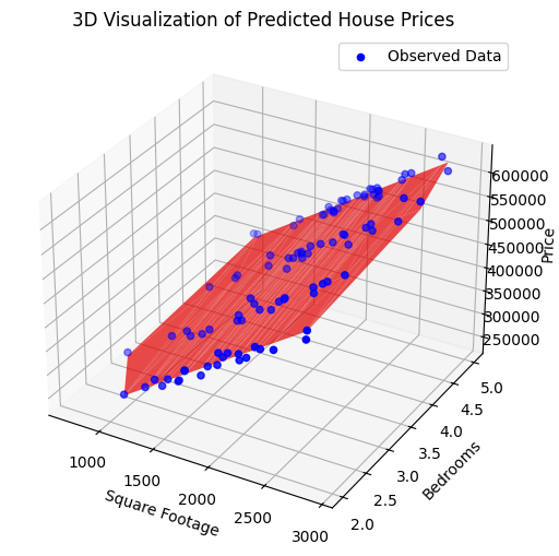
Visualization:
- A 3D scatter plot shows observed data points (blue dots).
- The red surface represents the predicted house prices based on the model.
Key Outputs
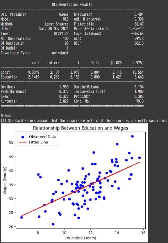
- Regression Summary:
- $Coefficients$: Show how house prices change with each feature.
- $R$-$squared$: Measures how well the model explains the variability in house prices.
                            OLS Regression Results
==============================================================================
Dep. Variable:                  Price   R-squared:                       0.984
Model:                            OLS   Adj. R-squared:                  0.984
Method:                 Least Squares   F-statistic:                     3049.
Date:                Sun, 01 Dec 2024   Prob (F-statistic):           2.77e-88
Time:                        03:00:00   Log-Likelihood:                -1060.8
No. Observations:                 100   AIC:                             2128.
Df Residuals:                      97   BIC:                             2135.
Df Model:                           2
Covariance Type:            nonrobust
=================================================================================
                    coef    std err          t      P>|t|      [0.025      0.975]
---------------------------------------------------------------------------------
const          4.882e+04   5331.911      9.157      0.000    3.82e+04    5.94e+04
SquareFootage   152.0480      2.201     69.074      0.000     147.679     156.417
Bedrooms       2.954e+04    868.797     33.999      0.000    2.78e+04    3.13e+04
==============================================================================
Omnibus:                        7.854   Durbin-Watson:                   2.034
Prob(Omnibus):                  0.020   Jarque-Bera (JB):                8.131
Skew:                           0.502   Prob(JB):                       0.0172
Kurtosis:                       3.971   Cond. No.                     1.08e+04
==============================================================================

Notes:
[1] Standard Errors assume that the covariance matrix of the errors is correctly specified.
[2] The condition number is large, 1.08e+04. This might indicate that there are
strong multicollinearity or other numerical problems.
- 3D Plot:
- The blue points are the actual data.
- The red plane shows the predicted relationship, helping to visualize the regression fit.
This example can be extended to include feature scaling, regularization (e.g., Ridge or Lasso regression), or additional predictors like location or age of the house.