Example Problem
We aim to simulate a simplified BoP analysis to understand the interactions between the Current Account (CA), Capital Account (KA), and the Financial Account (FA).
Problem
- The Current Account (CA) records trade in goods and services, income, and transfers.
- The Capital Account (KA) reflects capital transfers and acquisition/disposal of non-produced assets.
- The Financial Account (FA) captures investments in financial assets.
By the BoP identity:
$$
\text{CA} + \text{KA} + \text{FA} = 0
$$
We will simulate and visualize:
- Changes in the CA due to trade balance adjustments.
- How these changes are offset by the KA and FA to maintain equilibrium.
Python Code
1 | import numpy as np |
Explanation
- Current Account Dynamics:
- Adjustments in trade balance affect the CA over time.
- BoP Equilibrium:
- The KA and FA adjust to ensure that the BoP identity $(\text{CA} + \text{KA} + \text{FA} = 0)$ holds.
- Assumptions:
- The KA remains constant for simplicity.
- Changes in the CA are offset entirely by the FA.
Results
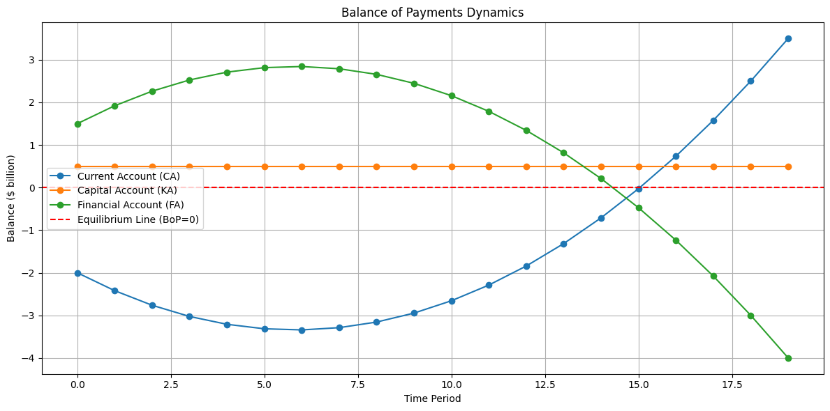
- The graph shows how the Current Account evolves due to trade balance changes.
- The Financial Account responds dynamically to maintain BoP equilibrium.
- The Capital Account remains constant, highlighting its lesser role in this simplified example.
This example illustrates the balancing act within the BoP framework, showing the interdependence of its components.