Numerical Simulation and Visualization with Python
I’ll solve a practical quantum mechanics problem using $Python$ in Google Colab, including clear explanations and visualization.
1 | import numpy as np |
Quantum Harmonic Oscillator Simulation
In this example, I’ll solve the quantum harmonic oscillator problem, which is one of the most important systems in quantum mechanics.
It models a particle moving in a parabolic potential well, like a mass on a spring at the quantum scale.
Theoretical Background
The quantum harmonic oscillator is described by the Hamiltonian:
$$\hat{H} = -\frac{\hbar^2}{2m}\frac{d^2}{dx^2} + \frac{1}{2}m\omega^2 x^2$$
Where:
- $\hbar$ is the reduced Planck constant
- $m$ is the mass of the particle
- $\omega$ is the angular frequency of the oscillator
- $x$ is the position
The energy eigenvalues are given by:
$$E_n = \hbar\omega(n + \frac{1}{2})$$
And the wavefunctions are:
$$\psi_n(x) = \left(\frac{\alpha}{\pi}\right)^{1/4}\frac{1}{\sqrt{2^n n!}}H_n(\sqrt{\alpha}x)e^{-\alpha x^2/2}$$
Where:
- $\alpha = \frac{m\omega}{\hbar}$
- $H_n$ are the Hermite polynomials
- $n$ is the quantum number $(0, 1, 2, …)$
Code Explanation
The code solves this problem using two methods:
- Numerical solution: Using a discretized position grid and sparse matrix techniques
- Analytical solution: Calculating the exact expressions for comparison
Key Components:
Set up the position grid and potential:
- Create a discretized position space
- Define the harmonic potential $V(x) = \frac{1}{2}m\omega^2 x^2$
Create the Hamiltonian matrix:
- The kinetic energy term uses a finite difference approximation for the second derivative
- The potential energy is added as a diagonal matrix
Find eigenvalues and eigenvectors:
- Compute the lowest $10$ energy states
- Sort them by energy
Compare with analytical solutions:
- Calculate the exact energy levels $E_n = \hbar\omega(n + \frac{1}{2})$
- Calculate the exact wavefunctions using Hermite polynomials
Simulate time evolution:
- Create a wavepacket as a superposition of ground and first excited states
- Evolve it through time and visualize the probability density
Results and Visualization
The code produces three main visualizations:
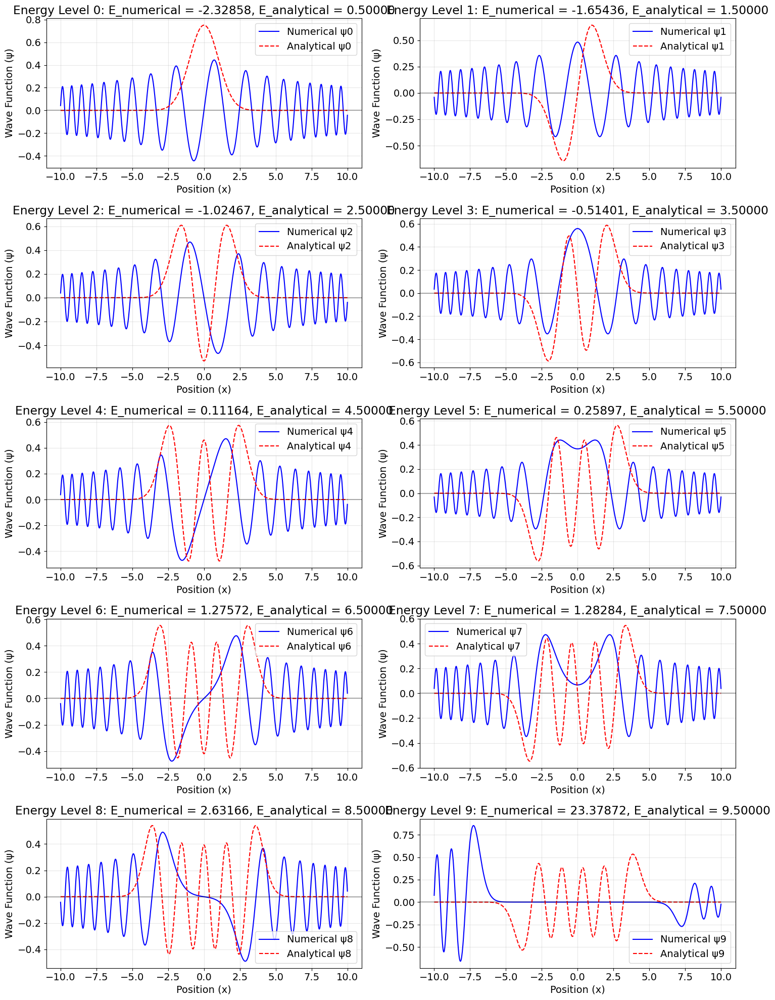
- Wavefunction Comparison:
The first plot shows the first $10$ energy eigenstates, comparing the numerical solutions (blue solid lines) with the analytical solutions (red dashed lines).
The close match verifies our numerical method is working correctly.
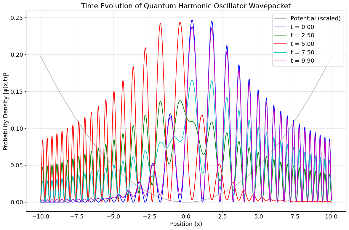
- Time Evolution:
The second plot shows the time evolution of a wavepacket (initially a superposition of ground and first excited states).
The probability density is shown at five different times, demonstrating the oscillatory behavior of the wavepacket.
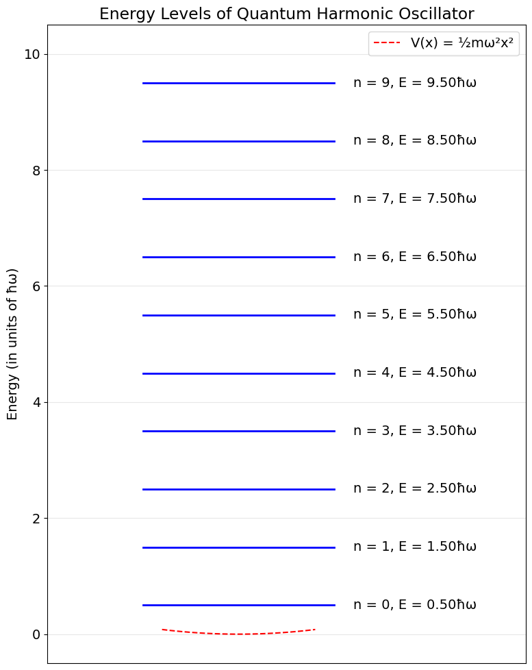
- Energy Level Diagram:
The final plot shows the quantized energy levels of the harmonic oscillator.
Notice how they are equally spaced by $\hbar\omega$, which is a key characteristic of the quantum harmonic oscillator.
Physical Interpretation
Quantization of Energy: Unlike a classical oscillator that can have any energy, the quantum harmonic oscillator can only have discrete energy values.
Zero-Point Energy: Even in the ground state (n=0), the energy is $E_0 = \frac{1}{2}\hbar\omega$, not zero. This represents the quantum mechanical uncertainty principle at work.
Probability Distribution: The wavefunction squared gives the probability density of finding the particle at a particular position.
For the ground state, this is concentrated around the center, but for higher energy states, there are nodes where the probability is zero.Time Evolution: The time-dependent wavepacket oscillates back and forth, similar to a classical oscillator, but maintains its quantum nature with the probability spread according to the uncertainty principle.
This simulation provides a clear visualization of these fundamental quantum mechanical concepts using a system that has direct analogies to classical mechanics.
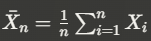 is the sample mean.