import numpy as np
import matplotlib.pyplot as plt
import torch
import torch.nn as nn
import torch.optim as optim

# Set random seed for reproducibility
torch.manual_seed(42)
np.random.seed(42)

# Generate synthetic data
x = np.linspace(0, 1, 100)
y_true = np.sin(2 * np.pi * x)
y_noisy = y_true + 0.1 * np.random.randn(*x.shape)

# Convert to PyTorch tensors
x_tensor = torch.tensor(x, dtype=torch.float32).unsqueeze(1)
y_tensor = torch.tensor(y_noisy, dtype=torch.float32).unsqueeze(1)

# Define a simple feedforward neural network
class Net(nn.Module):
    def __init__(self):
        super(Net, self).__init__()
        self.net = nn.Sequential(
            nn.Linear(1, 32),
            nn.ReLU(),
            nn.Linear(32, 32),
            nn.ReLU(),
            nn.Linear(32, 1)
        )

    def forward(self, x):
        return self.net(x)

model = Net()

# Define loss and optimizer with momentum
criterion = nn.MSELoss()
optimizer = optim.SGD(model.parameters(), lr=0.1, momentum=0.9)

# Training loop
epochs = 500
losses = []

for epoch in range(epochs):
    model.train()
    optimizer.zero_grad()
    outputs = model(x_tensor)
    loss = criterion(outputs, y_tensor)
    loss.backward()
    optimizer.step()
    losses.append(loss.item())

# Predictions
model.eval()
with torch.no_grad():
    predictions = model(x_tensor).numpy()

# Plot loss curve
plt.figure(figsize=(10, 4))
plt.subplot(1, 2, 1)
plt.plot(losses)
plt.title("Training Loss")
plt.xlabel("Epoch")
plt.ylabel("MSE Loss")
plt.grid(True)

# Plot predictions vs true function
plt.subplot(1, 2, 2)
plt.scatter(x, y_noisy, label="Noisy Data", alpha=0.6)
plt.plot(x, y_true, label="True Function", linestyle="dashed")
plt.plot(x, predictions, label="NN Prediction", color="red")
plt.title("Function Approximation")
plt.xlabel("x")
plt.ylabel("y")
plt.legend()
plt.grid(True)
plt.tight_layout()
plt.show()

import numpy as np
import matplotlib.pyplot as plt
from scipy.optimize import minimize
import pandas as pd

# Define power plant characteristics
plants = {
    'Coal': {
        'capacity_min': 200,  # MW
        'capacity_max': 800,  # MW
        'marginal_cost': 25,  # $/MWh
        'fixed_cost': 5000,   # $/h when operating
        'ramp_rate': 50,      # MW/h maximum change
        'efficiency': 0.35    # 35% efficiency
    },
    'Gas': {
        'capacity_min': 100,  # MW
        'capacity_max': 500,  # MW
        'marginal_cost': 45,  # $/MWh
        'fixed_cost': 2000,   # $/h when operating
        'ramp_rate': 200,     # MW/h maximum change
        'efficiency': 0.45    # 45% efficiency
    },
    'Peaker': {
        'capacity_min': 0,    # MW (can be completely shut down)
        'capacity_max': 200,  # MW
        'marginal_cost': 80,  # $/MWh
        'fixed_cost': 500,    # $/h when operating
        'ramp_rate': 150,     # MW/h maximum change
        'efficiency': 0.38    # 38% efficiency
    }
}

# Generate realistic 24-hour demand profile (typical summer day)
hours = np.arange(24)
base_demand = 800  # MW base load
peak_demand = 1200  # MW peak demand

# Create demand curve with morning and evening peaks
demand_profile = base_demand + (peak_demand - base_demand) * (
    0.3 * np.sin(2 * np.pi * (hours - 6) / 24) ** 2 +  # Morning peak
    0.7 * np.sin(2 * np.pi * (hours - 18) / 24) ** 2    # Evening peak
)

# Add some realistic noise
np.random.seed(42)
demand_profile += np.random.normal(0, 20, 24)
demand_profile = np.maximum(demand_profile, 600)  # Minimum demand floor

print("24-Hour Electricity Demand Profile:")
for i, demand in enumerate(demand_profile):
    print(f"Hour {i:2d}: {demand:6.1f} MW")

# Cost function for each plant
def plant_cost(power, plant_name):
    """Calculate total cost for a plant given power output"""
    if power <= 0:
        return 0
    
    plant = plants[plant_name]
    # Quadratic cost function: Fixed cost + marginal cost * power + quadratic term
    variable_cost = plant['marginal_cost'] * power + 0.01 * power**2
    fixed_cost = plant['fixed_cost'] if power > 0 else 0
    
    return fixed_cost + variable_cost

# Objective function for optimization
def total_cost(x):
    """Calculate total system cost for all plants across all hours"""
    # Reshape optimization variable: x = [coal_powers, gas_powers, peaker_powers]
    n_hours = 24
    coal_powers = x[0:n_hours]
    gas_powers = x[n_hours:2*n_hours]
    peaker_powers = x[2*n_hours:3*n_hours]
    
    total = 0
    for t in range(n_hours):
        total += plant_cost(coal_powers[t], 'Coal')
        total += plant_cost(gas_powers[t], 'Gas')
        total += plant_cost(peaker_powers[t], 'Peaker')
    
    return total

# Constraint functions
def power_balance_constraint(x):
    """Ensure power generation meets demand at each hour"""
    n_hours = 24
    coal_powers = x[0:n_hours]
    gas_powers = x[n_hours:2*n_hours]
    peaker_powers = x[2*n_hours:3*n_hours]
    
    # Return difference between generation and demand (should be zero)
    return coal_powers + gas_powers + peaker_powers - demand_profile

def ramp_rate_constraints(x):
    """Ensure power plants don't change output too quickly"""
    n_hours = 24
    constraints = []
    
    # Check ramp rates for each plant type
    plant_names = ['Coal', 'Gas', 'Peaker']
    for i, plant_name in enumerate(plant_names):
        powers = x[i*n_hours:(i+1)*n_hours]
        ramp_limit = plants[plant_name]['ramp_rate']
        
        for t in range(1, n_hours):
            # Constraint: |P(t) - P(t-1)| <= ramp_rate
            # Implemented as two constraints: P(t) - P(t-1) <= ramp_rate and P(t-1) - P(t) <= ramp_rate
            constraints.append(ramp_limit - (powers[t] - powers[t-1]))
            constraints.append(ramp_limit - (powers[t-1] - powers[t]))
    
    return np.array(constraints)

# Set up bounds for each variable (capacity constraints)
bounds = []
for plant_name in ['Coal', 'Gas', 'Peaker']:
    for _ in range(24):  # 24 hours
        bounds.append((plants[plant_name]['capacity_min'], 
                      plants[plant_name]['capacity_max']))

# Initial guess: distribute demand proportionally
initial_guess = []
total_capacity = sum(plants[p]['capacity_max'] for p in plants.keys())
for plant_name in ['Coal', 'Gas', 'Peaker']:
    plant_share = plants[plant_name]['capacity_max'] / total_capacity
    for demand in demand_profile:
        initial_power = demand * plant_share
        # Ensure initial guess is within bounds
        initial_power = max(plants[plant_name]['capacity_min'], 
                          min(initial_power, plants[plant_name]['capacity_max']))
        initial_guess.append(initial_power)

# Define constraints for the optimizer
constraints = [
    {'type': 'eq', 'fun': power_balance_constraint},
    {'type': 'ineq', 'fun': ramp_rate_constraints}
]

print("\nSolving economic dispatch optimization...")
print("This may take a moment...")

# Solve the optimization problem
result = minimize(
    total_cost,
    initial_guess,
    method='SLSQP',
    bounds=bounds,
    constraints=constraints,
    options={'maxiter': 1000, 'ftol': 1e-6}
)

if not result.success:
    print(f"Optimization failed: {result.message}")
else:
    print(f"Optimization successful!")
    print(f"Total daily cost: ${result.fun:,.2f}")

# Extract results
optimal_solution = result.x
n_hours = 24
coal_schedule = optimal_solution[0:n_hours]
gas_schedule = optimal_solution[n_hours:2*n_hours]
peaker_schedule = optimal_solution[2*n_hours:3*n_hours]

# Create results DataFrame
results_df = pd.DataFrame({
    'Hour': hours,
    'Demand_MW': demand_profile,
    'Coal_MW': coal_schedule,
    'Gas_MW': gas_schedule,
    'Peaker_MW': peaker_schedule,
    'Total_Generation_MW': coal_schedule + gas_schedule + peaker_schedule
})

# Calculate hourly costs
hourly_costs = []
for t in range(24):
    hour_cost = (plant_cost(coal_schedule[t], 'Coal') + 
                 plant_cost(gas_schedule[t], 'Gas') + 
                 plant_cost(peaker_schedule[t], 'Peaker'))
    hourly_costs.append(hour_cost)

results_df['Hourly_Cost_$'] = hourly_costs

print("\nOptimal Generation Schedule:")
print(results_df.round(1))

# Calculate summary statistics
total_generation = {
    'Coal': np.sum(coal_schedule),
    'Gas': np.sum(gas_schedule),
    'Peaker': np.sum(peaker_schedule)
}

print(f"\nDaily Generation Summary:")
for plant, total in total_generation.items():
    percentage = 100 * total / np.sum(demand_profile)
    avg_cost = plants[plant]['marginal_cost']
    print(f"{plant:7s}: {total:6.1f} MWh ({percentage:4.1f}%) - Avg Cost: ${avg_cost}/MWh")

print(f"\nTotal Daily Demand: {np.sum(demand_profile):6.1f} MWh")
print(f"Total Daily Cost: ${result.fun:,.2f}")
print(f"Average Cost per MWh: ${result.fun/np.sum(demand_profile):.2f}")

# Plotting results
fig, ((ax1, ax2), (ax3, ax4)) = plt.subplots(2, 2, figsize=(15, 12))

# Plot 1: Generation Schedule
ax1.plot(hours, demand_profile, 'k-', linewidth=3, label='Demand', marker='o')
ax1.plot(hours, coal_schedule, 'brown', linewidth=2, label='Coal', marker='s')
ax1.plot(hours, gas_schedule, 'blue', linewidth=2, label='Natural Gas', marker='^')
ax1.plot(hours, peaker_schedule, 'red', linewidth=2, label='Peaker', marker='d')

ax1.set_xlabel('Hour of Day')
ax1.set_ylabel('Power (MW)')
ax1.set_title('Optimal Generation Schedule vs Demand')
ax1.legend()
ax1.grid(True, alpha=0.3)
ax1.set_xticks(range(0, 24, 2))

# Plot 2: Stacked Generation
ax2.fill_between(hours, 0, coal_schedule, alpha=0.7, color='brown', label='Coal')
ax2.fill_between(hours, coal_schedule, coal_schedule + gas_schedule, 
                alpha=0.7, color='blue', label='Natural Gas')
ax2.fill_between(hours, coal_schedule + gas_schedule, 
                coal_schedule + gas_schedule + peaker_schedule,
                alpha=0.7, color='red', label='Peaker')
ax2.plot(hours, demand_profile, 'k-', linewidth=2, label='Demand')

ax2.set_xlabel('Hour of Day')
ax2.set_ylabel('Power (MW)')
ax2.set_title('Generation Mix (Stacked)')
ax2.legend()
ax2.grid(True, alpha=0.3)
ax2.set_xticks(range(0, 24, 2))

# Plot 3: Hourly Costs
ax3.bar(hours, hourly_costs, alpha=0.7, color='green')
ax3.set_xlabel('Hour of Day')
ax3.set_ylabel('Hourly Cost ($)')
ax3.set_title('Hourly Generation Costs')
ax3.grid(True, alpha=0.3)
ax3.set_xticks(range(0, 24, 2))

# Plot 4: Generation Mix Pie Chart
total_gen = [total_generation[plant] for plant in ['Coal', 'Gas', 'Peaker']]
colors = ['brown', 'blue', 'red']
ax4.pie(total_gen, labels=['Coal', 'Natural Gas', 'Peaker'], 
        colors=colors, autopct='%1.1f%%', startangle=90)
ax4.set_title('Daily Generation Mix')

plt.tight_layout()
plt.show()

# Additional analysis: Marginal costs
print(f"\nMarginal Cost Analysis:")
print(f"Coal marginal cost: ${plants['Coal']['marginal_cost']}/MWh")
print(f"Gas marginal cost: ${plants['Gas']['marginal_cost']}/MWh") 
print(f"Peaker marginal cost: ${plants['Peaker']['marginal_cost']}/MWh")

# Calculate capacity factors
print(f"\nCapacity Factors:")
for plant_name in ['Coal', 'Gas', 'Peaker']:
    if plant_name == 'Coal':
        generation = coal_schedule
    elif plant_name == 'Gas':
        generation = gas_schedule
    else:
        generation = peaker_schedule
    
    max_capacity = plants[plant_name]['capacity_max']
    avg_generation = np.mean(generation)
    capacity_factor = avg_generation / max_capacity * 100
    print(f"{plant_name:7s}: {capacity_factor:5.1f}% (Avg: {avg_generation:5.1f} MW)")

import numpy as np
import matplotlib.pyplot as plt
from scipy.integrate import odeint
from scipy.optimize import minimize

# Define the second-order system
def system(state, t, Kp, Ki, Kd, setpoint):
    x, x_dot, integral = state
    error = setpoint - x
    u = Kp * error + Ki * integral + Kd * (-x_dot)
    m, c, k = 1.0, 0.2, 1.0  # Mass, damping, spring constant
    x_ddot = (u - c * x_dot - k * x) / m
    return [x_dot, x_ddot, error]

# Simulate the system for given PID parameters
def simulate_pid(params, t, setpoint=1.0):
    Kp, Ki, Kd = params
    initial_state = [0.0, 0.0, 0.0]  # Initial position, velocity, integral
    states = odeint(system, initial_state, t, args=(Kp, Ki, Kd, setpoint))
    return states[:, 0], states[:, 2]  # Return position and integral of error

# Objective function for optimization (minimize ITAE)
def objective(params, t, setpoint=1.0):
    y, integral = simulate_pid(params, t, setpoint)
    error = setpoint - y
    itae = np.trapz(t * np.abs(error), t)
    return itae

# Optimization and simulation
t = np.linspace(0, 10, 1000)
initial_params = [1.0, 0.1, 0.1]  # Initial guess for Kp, Ki, Kd
bounds = [(0, 10), (0, 10), (0, 10)]  # Bounds for Kp, Ki, Kd
result = minimize(objective, initial_params, args=(t,), bounds=bounds)

# Get optimized parameters
Kp_opt, Ki_opt, Kd_opt = result.x
y_opt, _ = simulate_pid(result.x, t)

# Simulate with initial parameters for comparison
y_init, _ = simulate_pid(initial_params, t)

# Plot results
plt.figure(figsize=(10, 6))
plt.plot(t, y_opt, label=f'Optimized: Kp={Kp_opt:.2f}, Ki={Ki_opt:.2f}, Kd={Kd_opt:.2f}')
plt.plot(t, y_init, label=f'Initial: Kp={initial_params[0]}, Ki={initial_params[1]}, Kd={initial_params[2]}')
plt.plot(t, [1.0]*len(t), 'k--', label='Setpoint')
plt.xlabel('Time (s)')
plt.ylabel('Output')
plt.title('PID Controller Response: Initial vs Optimized')
plt.legend()
plt.grid(True)
plt.show()

print(f"Optimized Parameters: Kp={Kp_opt:.2f}, Ki={Ki_opt:.2f}, Kd={Kd_opt:.2f}")
print(f"ITAE (Optimized): {objective(result.x, t):.2f}")
print(f"ITAE (Initial): {objective(initial_params, t):.2f}")

import numpy as np
import matplotlib.pyplot as plt
from scipy.optimize import minimize_scalar

# Parameters
F = 1.0        # Bioavailability
D = 500        # Dose in mg
ka = 1.5       # Absorption rate constant (1/hr)
ke = 0.3       # Elimination rate constant (1/hr)
Vd = 40        # Volume of distribution (L)
t_end = 72     # Total simulation time (hr)
dose_count = 10

# Target therapeutic range
C_min = 10     # Minimum effective concentration (mg/L)
C_max = 20     # Maximum safe concentration (mg/L)

def concentration_single_dose(t):
    """Concentration after a single oral dose at time t"""
    return (F * D * ka) / (Vd * (ka - ke)) * (np.exp(-ke * t) - np.exp(-ka * t))

def concentration_multiple_doses(tau):
    """Simulate multiple doses given at interval tau"""
    t = np.linspace(0, t_end, 1000)
    C = np.zeros_like(t)
    for n in range(dose_count):
        tn = n * tau
        C += concentration_single_dose(np.clip(t - tn, 0, None))
    return t, C

def objective(tau):
    """Objective: Penalize time outside therapeutic range"""
    t, C = concentration_multiple_doses(tau)
    penalty = np.sum((C < C_min) * (C_min - C)**2 + (C > C_max) * (C - C_max)**2)
    return penalty

# Optimization
result = minimize_scalar(objective, bounds=(4, 24), method='bounded')
optimal_tau = result.x
print(f"Optimal dosing interval: {optimal_tau:.2f} hours")

# Final simulation with optimal tau
t, C = concentration_multiple_doses(optimal_tau)

plt.figure(figsize=(12, 5))
plt.plot(t, C, label='Drug Concentration')
plt.axhline(C_min, color='green', linestyle='--', label='Min Effective (10 mg/L)')
plt.axhline(C_max, color='red', linestyle='--', label='Max Safe (20 mg/L)')
plt.title(f"Optimized Drug Dosing (Interval: {optimal_tau:.2f} hr)")
plt.xlabel('Time (hours)')
plt.ylabel('Concentration (mg/L)')
plt.legend()
plt.grid(True)
plt.show()

import numpy as np
import matplotlib.pyplot as plt

# Set random seed for reproducibility
np.random.seed(42)

# Depot location
depot = np.array([50, 50])

# Generate random delivery locations
n_deliveries = 10
locations = np.random.rand(n_deliveries, 2) * 100  # 100x100 area

# Calculate energy usage for each round trip (Euclidean distance * 2)
def calculate_total_energy(depot, locations):
    distances = np.linalg.norm(locations - depot, axis=1)
    return np.sum(distances * 2)

total_energy = calculate_total_energy(depot, locations)

print(f"Total round-trip energy usage (arbitrary units): {total_energy:.2f}")

# Plot depot and delivery locations
plt.figure(figsize=(8, 8))
plt.scatter(*depot, color='red', label='Depot', s=100)
plt.scatter(locations[:, 0], locations[:, 1], label='Deliveries', s=60)

# Draw lines for round trips
for loc in locations:
    plt.plot([depot[0], loc[0]], [depot[1], loc[1]], color='gray', linestyle='--', alpha=0.6)

plt.title('Electric Delivery Routes')
plt.xlabel('X Coordinate')
plt.ylabel('Y Coordinate')
plt.grid(True)
plt.legend()
plt.show()

from sklearn.cluster import KMeans

# Assume we use 3 trucks and cluster the deliveries
kmeans = KMeans(n_clusters=3, random_state=42)
kmeans.fit(locations)
labels = kmeans.labels_
centroids = kmeans.cluster_centers_

# Recalculate energy: depot to centroid and back (simulating drop-off and collection hub)
cluster_energy = np.sum([np.linalg.norm(c - depot) * 2 for c in centroids])

print(f"Energy usage with clustered deliveries: {cluster_energy:.2f}")

plt.bar(['Individual Trips', 'Clustered'], [total_energy, cluster_energy], color=['blue', 'green'])
plt.title('Energy Usage Comparison')
plt.ylabel('Energy Units')
plt.show()

import numpy as np
import matplotlib.pyplot as plt
import seaborn as sns
from scipy.optimize import linprog
import pandas as pd
from matplotlib.patches import Rectangle
import warnings
warnings.filterwarnings('ignore')

# Set random seed for reproducibility
np.random.seed(42)

# Problem Setup: 10 potential locations for renewable energy installation
n_locations = 10
location_names = [f'Site_{i+1}' for i in range(n_locations)]

# Generate realistic data for each location
# Wind speed data (m/s) - affects wind turbine efficiency
wind_speeds = np.random.uniform(4.5, 12.0, n_locations)

# Solar irradiance data (kWh/m²/day) - affects solar panel efficiency  
solar_irradiance = np.random.uniform(3.5, 6.5, n_locations)

# Wind turbine specifications
turbine_capacity = 2.5  # MW per turbine
turbine_cost = 3.0      # Million $ per turbine
turbine_maintenance = 0.1  # Million $ per year per turbine

# Solar panel specifications  
solar_capacity_per_unit = 1.0  # MW per solar unit
solar_cost = 1.5              # Million $ per solar unit
solar_maintenance = 0.05      # Million $ per year per solar unit

# Grid connection costs (varies by location)
grid_connection_cost = np.random.uniform(0.2, 0.8, n_locations)

# Calculate energy output coefficients
# Wind energy output: P = 0.5 * ρ * A * v³ * Cp (simplified)
# We'll use a simplified efficiency curve
def wind_efficiency(wind_speed):
    """Calculate wind turbine efficiency based on wind speed"""
    if wind_speed < 3:
        return 0
    elif wind_speed < 12:
        return 0.35 * (wind_speed / 12) ** 3
    else:
        return 0.35

# Solar efficiency is more linear with irradiance
def solar_efficiency(irradiance):
    """Calculate solar panel efficiency based on irradiance"""
    return 0.18 * (irradiance / 5.0)

# Calculate annual energy output for each location (GWh/year)
wind_output = np.array([wind_efficiency(ws) * turbine_capacity * 8760 / 1000 
                       for ws in wind_speeds])
solar_output = np.array([solar_efficiency(si) * solar_capacity_per_unit * 8760 / 1000 
                        for si in solar_irradiance])

# Total costs per installation (including 5-year maintenance)
wind_total_cost = turbine_cost + 5 * turbine_maintenance + grid_connection_cost
solar_total_cost = solar_cost + 5 * solar_maintenance + grid_connection_cost

# Budget constraint
total_budget = 50.0  # Million $

print("=== Renewable Energy Optimization Problem ===")
print(f"Budget: ${total_budget} million")
print(f"Number of potential sites: {n_locations}")
print(f"Wind turbine capacity: {turbine_capacity} MW")
print(f"Solar unit capacity: {solar_capacity_per_unit} MW")
print("\n=== Location Data ===")

# Create comprehensive data table
data_table = pd.DataFrame({
    'Location': location_names,
    'Wind_Speed_ms': np.round(wind_speeds, 2),
    'Solar_Irradiance_kWh_m2_day': np.round(solar_irradiance, 2),
    'Wind_Output_GWh_year': np.round(wind_output, 2),
    'Solar_Output_GWh_year': np.round(solar_output, 2),
    'Wind_Cost_Million': np.round(wind_total_cost, 2),
    'Solar_Cost_Million': np.round(solar_total_cost, 2),
    'Grid_Connection_Million': np.round(grid_connection_cost, 2)
})

print(data_table.to_string(index=False))

# Mathematical Formulation
print("\n=== Mathematical Formulation ===")
print("Objective Function:")
print("Maximize: Σ(wind_output[i] * x_wind[i] + solar_output[i] * x_solar[i])")
print("\nSubject to:")
print("Σ(wind_cost[i] * x_wind[i] + solar_cost[i] * x_solar[i]) ≤ Budget")
print("x_wind[i], x_solar[i] ∈ {0, 1} for all i")

# Since scipy.optimize.linprog doesn't handle integer programming directly,
# we'll use a relaxed LP and then apply rounding heuristics
# For exact integer solutions, specialized solvers like PuLP would be better

# Prepare linear programming formulation
# Variables: [x_wind_0, x_wind_1, ..., x_wind_9, x_solar_0, x_solar_1, ..., x_solar_9]
c = np.concatenate([-wind_output, -solar_output])  # Negative for maximization
A_ub = np.concatenate([wind_total_cost, solar_total_cost]).reshape(1, -1)
b_ub = np.array([total_budget])

# Bounds: 0 ≤ x ≤ 1 for relaxed problem
bounds = [(0, 1) for _ in range(2 * n_locations)]

# Solve relaxed linear program
print("\n=== Solving Optimization Problem ===")
result = linprog(c, A_ub=A_ub, b_ub=b_ub, bounds=bounds, method='highs')

if result.success:
    print("Optimization successful!")
    
    # Extract solutions
    x_wind_relaxed = result.x[:n_locations]
    x_solar_relaxed = result.x[n_locations:]
    
    # Apply rounding heuristic for integer solution
    # Sort by efficiency ratio (output/cost) and select greedily
    wind_efficiency_ratio = wind_output / wind_total_cost
    solar_efficiency_ratio = solar_output / solar_total_cost
    
    # Create candidate list with efficiency ratios
    candidates = []
    for i in range(n_locations):
        candidates.append(('wind', i, wind_efficiency_ratio[i], wind_total_cost[i], wind_output[i]))
        candidates.append(('solar', i, solar_efficiency_ratio[i], solar_total_cost[i], solar_output[i]))
    
    # Sort by efficiency ratio (descending)
    candidates.sort(key=lambda x: x[2], reverse=True)
    
    # Greedy selection
    selected_wind = np.zeros(n_locations, dtype=int)
    selected_solar = np.zeros(n_locations, dtype=int)
    remaining_budget = total_budget
    total_output = 0
    
    print("\n=== Greedy Selection Process ===")
    for energy_type, location, ratio, cost, output in candidates:
        if cost <= remaining_budget:
            if energy_type == 'wind':
                selected_wind[location] = 1
            else:
                selected_solar[location] = 1
            remaining_budget -= cost
            total_output += output
            print(f"Selected: {energy_type.upper()} at {location_names[location]} "
                  f"(Efficiency: {ratio:.3f}, Cost: ${cost:.2f}M, Output: {output:.2f} GWh/year)")
    
    print(f"\nRemaining budget: ${remaining_budget:.2f} million")
    print(f"Total annual energy output: {total_output:.2f} GWh/year")
    
    # Calculate total investment
    total_investment = total_budget - remaining_budget
    print(f"Total investment: ${total_investment:.2f} million")
    
else:
    print("Optimization failed!")
    selected_wind = np.zeros(n_locations, dtype=int)
    selected_solar = np.zeros(n_locations, dtype=int)

# Create comprehensive results analysis
print("\n=== Final Solution Analysis ===")
solution_df = pd.DataFrame({
    'Location': location_names,
    'Wind_Selected': selected_wind,
    'Solar_Selected': selected_solar,
    'Wind_Speed': np.round(wind_speeds, 2),
    'Solar_Irradiance': np.round(solar_irradiance, 2),
    'Total_Output_GWh': np.round(
        selected_wind * wind_output + selected_solar * solar_output, 2),
    'Total_Cost_Million': np.round(
        selected_wind * wind_total_cost + selected_solar * solar_total_cost, 2)
})

print(solution_df.to_string(index=False))

# Visualization Section
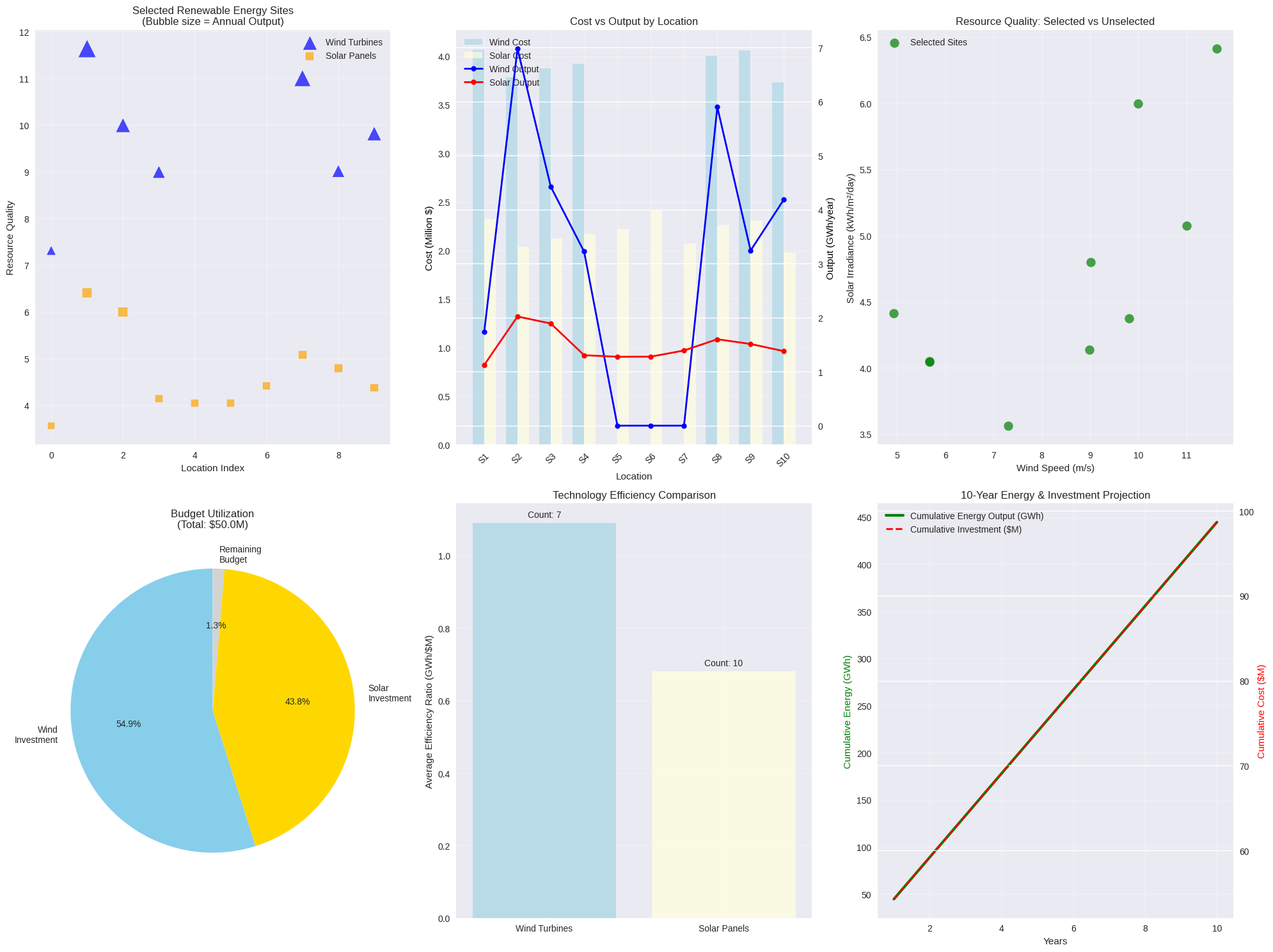
plt.style.use('seaborn-v0_8')
fig = plt.figure(figsize=(20, 15))

# 1. Location Overview Map-style Plot
ax1 = plt.subplot(2, 3, 1)
scatter_wind = ax1.scatter([i for i in range(n_locations) if selected_wind[i]], 
                         [wind_speeds[i] for i in range(n_locations) if selected_wind[i]],
                         s=[wind_output[i]*50 for i in range(n_locations) if selected_wind[i]], 
                         c='blue', alpha=0.7, label='Wind Turbines', marker='^')

scatter_solar = ax1.scatter([i for i in range(n_locations) if selected_solar[i]], 
                          [solar_irradiance[i] for i in range(n_locations) if selected_solar[i]],
                          s=[solar_output[i]*50 for i in range(n_locations) if selected_solar[i]], 
                          c='orange', alpha=0.7, label='Solar Panels', marker='s')

# Add unselected locations in gray
unselected_idx = [i for i in range(n_locations) 
                 if not selected_wind[i] and not selected_solar[i]]
if unselected_idx:
    ax1.scatter(unselected_idx, [wind_speeds[i] for i in unselected_idx],
               c='gray', alpha=0.3, s=30, label='Unselected')

ax1.set_xlabel('Location Index')
ax1.set_ylabel('Resource Quality')
ax1.set_title('Selected Renewable Energy Sites\n(Bubble size = Annual Output)')
ax1.legend()
ax1.grid(True, alpha=0.3)

# 2. Cost vs Output Analysis
ax2 = plt.subplot(2, 3, 2)
wind_costs = [wind_total_cost[i] if selected_wind[i] else 0 for i in range(n_locations)]
solar_costs = [solar_total_cost[i] if selected_solar[i] else 0 for i in range(n_locations)]
wind_outputs = [wind_output[i] if selected_wind[i] else 0 for i in range(n_locations)]
solar_outputs = [solar_output[i] if selected_solar[i] else 0 for i in range(n_locations)]

x_pos = np.arange(n_locations)
width = 0.35

bars1 = ax2.bar(x_pos - width/2, wind_costs, width, label='Wind Cost', color='lightblue', alpha=0.7)
bars2 = ax2.bar(x_pos + width/2, solar_costs, width, label='Solar Cost', color='lightyellow', alpha=0.7)

ax2_twin = ax2.twinx()
line1 = ax2_twin.plot(x_pos, wind_outputs, 'bo-', label='Wind Output', linewidth=2, markersize=6)
line2 = ax2_twin.plot(x_pos, solar_outputs, 'ro-', label='Solar Output', linewidth=2, markersize=6)

ax2.set_xlabel('Location')
ax2.set_ylabel('Cost (Million $)', color='black')
ax2_twin.set_ylabel('Output (GWh/year)', color='black')
ax2.set_title('Cost vs Output by Location')
ax2.set_xticks(x_pos)
ax2.set_xticklabels([f'S{i+1}' for i in range(n_locations)], rotation=45)

# Combine legends
lines1, labels1 = ax2.get_legend_handles_labels()
lines2, labels2 = ax2_twin.get_legend_handles_labels()
ax2.legend(lines1 + lines2, labels1 + labels2, loc='upper left')
ax2.grid(True, alpha=0.3)

# 3. Resource Quality Distribution
ax3 = plt.subplot(2, 3, 3)
selected_locations = [i for i in range(n_locations) 
                     if selected_wind[i] or selected_solar[i]]
unselected_locations = [i for i in range(n_locations) 
                       if not (selected_wind[i] or selected_solar[i])]

if selected_locations:
    ax3.scatter([wind_speeds[i] for i in selected_locations], 
               [solar_irradiance[i] for i in selected_locations],
               c='green', s=100, alpha=0.7, label='Selected Sites')

if unselected_locations:
    ax3.scatter([wind_speeds[i] for i in unselected_locations], 
               [solar_irradiance[i] for i in unselected_locations],
               c='red', s=100, alpha=0.7, label='Unselected Sites')

ax3.set_xlabel('Wind Speed (m/s)')
ax3.set_ylabel('Solar Irradiance (kWh/m²/day)')
ax3.set_title('Resource Quality: Selected vs Unselected')
ax3.legend()
ax3.grid(True, alpha=0.3)

# 4. Budget Utilization
ax4 = plt.subplot(2, 3, 4)
budget_categories = ['Wind\nInvestment', 'Solar\nInvestment', 'Remaining\nBudget']
budget_values = [
    np.sum(selected_wind * wind_total_cost),
    np.sum(selected_solar * solar_total_cost),
    remaining_budget
]
colors = ['skyblue', 'gold', 'lightgray']

wedges, texts, autotexts = ax4.pie(budget_values, labels=budget_categories, 
                                  autopct='%1.1f%%', startangle=90, colors=colors)
ax4.set_title(f'Budget Utilization\n(Total: ${total_budget}M)')

# 5. Efficiency Comparison
ax5 = plt.subplot(2, 3, 5)
efficiency_data = {
    'Technology': ['Wind Turbines', 'Solar Panels'],
    'Avg_Efficiency_Ratio': [
        np.mean([wind_efficiency_ratio[i] for i in range(n_locations) if selected_wind[i]]) 
        if np.sum(selected_wind) > 0 else 0,
        np.mean([solar_efficiency_ratio[i] for i in range(n_locations) if selected_solar[i]]) 
        if np.sum(selected_solar) > 0 else 0
    ],
    'Count': [np.sum(selected_wind), np.sum(selected_solar)]
}

bars = ax5.bar(efficiency_data['Technology'], efficiency_data['Avg_Efficiency_Ratio'], 
               color=['lightblue', 'lightyellow'], alpha=0.8)

# Add count labels on bars
for bar, count in zip(bars, efficiency_data['Count']):
    height = bar.get_height()
    ax5.text(bar.get_x() + bar.get_width()/2., height + 0.01,
             f'Count: {count}', ha='center', va='bottom')

ax5.set_ylabel('Average Efficiency Ratio (GWh/$M)')
ax5.set_title('Technology Efficiency Comparison')
ax5.grid(True, alpha=0.3)

# 6. Timeline Projection
ax6 = plt.subplot(2, 3, 6)
years = np.arange(1, 11)  # 10-year projection
annual_output = total_output
cumulative_output = annual_output * years
cumulative_investment = total_investment + np.arange(1, 11) * 0.1 * total_investment  # 10% annual maintenance

ax6.plot(years, cumulative_output, 'g-', linewidth=3, label='Cumulative Energy Output (GWh)')
ax6_twin = ax6.twinx()
ax6_twin.plot(years, cumulative_investment, 'r--', linewidth=2, label='Cumulative Investment ($M)')

ax6.set_xlabel('Years')
ax6.set_ylabel('Cumulative Energy (GWh)', color='green')
ax6_twin.set_ylabel('Cumulative Cost ($M)', color='red')
ax6.set_title('10-Year Energy & Investment Projection')
ax6.grid(True, alpha=0.3)

# Combine legends
lines1, labels1 = ax6.get_legend_handles_labels()
lines2, labels2 = ax6_twin.get_legend_handles_labels()
ax6.legend(lines1 + lines2, labels1 + labels2, loc='upper left')

plt.tight_layout()
plt.show()

# Mathematical Summary
print("\n" + "="*60)
print("MATHEMATICAL FORMULATION SUMMARY")
print("="*60)

print("\nObjective Function (Maximization):")
print("$$\\max \\sum_{i=1}^{n} \\left( E_{wind}^i \\cdot x_{wind}^i + E_{solar}^i \\cdot x_{solar}^i \\right)$$")

print("\nWhere:")
print("- $E_{wind}^i$: Annual wind energy output at location $i$")
print("- $E_{solar}^i$: Annual solar energy output at location $i$")  
print("- $x_{wind}^i$: Binary decision variable for wind installation at location $i$")
print("- $x_{solar}^i$: Binary decision variable for solar installation at location $i$")

print("\nConstraints:")
print("Budget Constraint:")
print("$$\\sum_{i=1}^{n} \\left( C_{wind}^i \\cdot x_{wind}^i + C_{solar}^i \\cdot x_{solar}^i \\right) \\leq B$$")

print("\nBinary Constraints:")
print("$$x_{wind}^i, x_{solar}^i \\in \\{0,1\\} \\quad \\forall i \\in \\{1,2,...,n\\}$$")

print(f"\nProblem Instance:")
print(f"- $n = {n_locations}$ (number of locations)")
print(f"- $B = {total_budget}$ million USD (budget)")
print(f"- Total variables: {2*n_locations} (binary)")

print(f"\nSolution Quality:")
print(f"- Total annual output: {total_output:.2f} GWh/year")
print(f"- Budget utilization: {(total_investment/total_budget)*100:.1f}%")
print(f"- Wind installations: {np.sum(selected_wind)}")
print(f"- Solar installations: {np.sum(selected_solar)}")
print(f"- Average ROI: {total_output/total_investment:.2f} GWh per million USD")

print("\n" + "="*60)
print("OPTIMIZATION COMPLETE")
print("="*60)

import numpy as np
import matplotlib.pyplot as plt
from scipy.optimize import minimize

# Given constants
P = 1000          # Load in N
L = 2.0           # Length in meters
rho = 7850        # Density of steel (kg/m^3)
g = 9.81          # Gravity (m/s^2)
sigma_yield = 250e6  # Yield stress in Pa
b = 0.05          # Fixed width in meters

# Objective function: weight of the beam
def weight(x):
    h = x[0]
    volume = b * h * L
    return rho * g * volume  # Weight = mass * gravity

# Constraint: maximum bending stress must be less than yield
def stress_constraint(x):
    h = x[0]
    sigma_max = 6 * P * L / (b * h**2)
    return sigma_yield - sigma_max

# Bounds and constraints
bounds = [(0.01, 0.5)]  # height h should be between 1cm and 50cm
constraints = [{'type': 'ineq', 'fun': stress_constraint}]

# Initial guess
x0 = [0.1]

# Run optimization
result = minimize(weight, x0, method='SLSQP', bounds=bounds, constraints=constraints)

# Extract result
h_opt = result.x[0]
w_opt = weight([h_opt])

print(f"Optimal height h = {h_opt:.4f} m")
print(f"Minimum weight = {w_opt:.2f} N")

def weight(x):
    h = x[0]
    volume = b * h * L
    return rho * g * volume

def stress_constraint(x):
    h = x[0]
    sigma_max = 6 * P * L / (b * h**2)
    return sigma_yield - sigma_max

h_vals = np.linspace(0.01, 0.5, 100)
weights = rho * g * b * h_vals * L
stresses = 6 * P * L / (b * h_vals**2)

fig, ax1 = plt.subplots()

ax1.set_xlabel('Height h (m)')
ax1.set_ylabel('Weight (N)', color='tab:blue')
ax1.plot(h_vals, weights, label='Weight', color='tab:blue')
ax1.tick_params(axis='y', labelcolor='tab:blue')

ax2 = ax1.twinx()
ax2.set_ylabel('Max Bending Stress (Pa)', color='tab:red')
ax2.plot(h_vals, stresses, label='Stress', color='tab:red')
ax2.axhline(sigma_yield, color='gray', linestyle='--', label='Yield Stress')
ax2.tick_params(axis='y', labelcolor='tab:red')

plt.title("Beam Weight and Stress vs Height")
fig.tight_layout()
plt.legend()
plt.grid(True)
plt.show()

import numpy as np
import matplotlib.pyplot as plt
import random
from collections import defaultdict
import seaborn as sns
from scipy.optimize import differential_evolution
import warnings
warnings.filterwarnings('ignore')

# Set random seed for reproducibility
np.random.seed(42)
random.seed(42)

class HPProteinFolder:
    """
    HP Model Protein Folding Optimizer
    
    This class implements a simplified protein folding model where:
    - H represents hydrophobic amino acids
    - P represents polar amino acids
    - Goal: Maximize hydrophobic contacts while avoiding collisions
    """
    
    def __init__(self, sequence):
        """
        Initialize the protein folder with an HP sequence
        
        Args:
            sequence (str): String of 'H' and 'P' characters representing the protein
        """
        self.sequence = sequence
        self.length = len(sequence)
        self.moves = [(0, 1), (1, 0), (0, -1), (-1, 0)]  # Up, Right, Down, Left
        self.move_names = ['U', 'R', 'D', 'L']
        
    def decode_folding(self, angles):
        """
        Convert angle representation to 2D coordinates
        
        Args:
            angles (list): List of angles (0-3) representing folding directions
            
        Returns:
            tuple: (coordinates, valid_folding_flag)
        """
        if len(angles) != self.length - 1:
            return None, False
            
        coordinates = [(0, 0)]  # Start at origin
        current_pos = (0, 0)
        occupied = {(0, 0)}
        
        for i, angle in enumerate(angles):
            # Convert continuous angle to discrete move
            move_idx = int(angle) % 4
            dx, dy = self.moves[move_idx]
            new_pos = (current_pos[0] + dx, current_pos[1] + dy)
            
            # Check for collision (self-intersection)
            if new_pos in occupied:
                return None, False
                
            coordinates.append(new_pos)
            occupied.add(new_pos)
            current_pos = new_pos
            
        return coordinates, True
    
    def calculate_energy(self, coordinates):
        """
        Calculate the energy of a folding configuration
        
        Energy = -1 * (number of H-H contacts that are adjacent in space but not in sequence)
        
        Args:
            coordinates (list): List of (x, y) coordinates for each amino acid
            
        Returns:
            float: Energy value (lower is better)
        """
        if coordinates is None:
            return float('inf')  # Invalid folding has infinite energy
            
        energy = 0
        
        # Check all pairs of amino acids
        for i in range(self.length):
            for j in range(i + 2, self.length):  # Skip adjacent in sequence
                # Only count H-H interactions
                if self.sequence[i] == 'H' and self.sequence[j] == 'H':
                    # Check if they are adjacent in 2D space
                    dist = abs(coordinates[i][0] - coordinates[j][0]) + abs(coordinates[i][1] - coordinates[j][1])
                    if dist == 1:  # Manhattan distance = 1 means adjacent
                        energy -= 1  # Favorable interaction
                        
        return energy
    
    def objective_function(self, angles):
        """
        Objective function for optimization
        
        Args:
            angles (array): Array of folding angles
            
        Returns:
            float: Energy to minimize
        """
        coordinates, valid = self.decode_folding(angles)
        if not valid:
            return 1000  # Heavy penalty for invalid folding
            
        return self.calculate_energy(coordinates)
    
    def optimize_folding(self, method='differential_evolution', max_iterations=1000):
        """
        Optimize protein folding using specified optimization method
        
        Args:
            method (str): Optimization method to use
            max_iterations (int): Maximum number of iterations
            
        Returns:
            tuple: (best_angles, best_energy, optimization_history)
        """
        bounds = [(0, 3.99) for _ in range(self.length - 1)]
        history = []
        
        def callback(xk, convergence=None):
            energy = self.objective_function(xk)
            history.append(energy)
            return False
        
        if method == 'differential_evolution':
            result = differential_evolution(
                self.objective_function,
                bounds,
                maxiter=max_iterations // 10,
                popsize=15,
                callback=callback,
                seed=42
            )
            best_angles = result.x
            best_energy = result.fun
            
        return best_angles, best_energy, history
    
    def monte_carlo_optimization(self, max_iterations=10000, temperature=1.0, cooling_rate=0.995):
        """
        Monte Carlo optimization with simulated annealing
        
        Args:
            max_iterations (int): Maximum number of iterations
            temperature (float): Initial temperature
            cooling_rate (float): Temperature cooling rate
            
        Returns:
            tuple: (best_angles, best_energy, history)
        """
        current_angles = [random.uniform(0, 3.99) for _ in range(self.length - 1)]
        current_energy = self.objective_function(current_angles)
        
        best_angles = current_angles.copy()
        best_energy = current_energy
        history = [current_energy]
        
        temp = temperature
        
        for iteration in range(max_iterations):
            # Generate neighbor solution
            new_angles = current_angles.copy()
            idx = random.randint(0, len(new_angles) - 1)
            new_angles[idx] = random.uniform(0, 3.99)
            
            new_energy = self.objective_function(new_angles)
            
            # Accept or reject based on Metropolis criterion
            if new_energy < current_energy or random.random() < np.exp(-(new_energy - current_energy) / temp):
                current_angles = new_angles
                current_energy = new_energy
                
                if current_energy < best_energy:
                    best_angles = current_angles.copy()
                    best_energy = current_energy
            
            history.append(best_energy)
            temp *= cooling_rate
            
            if iteration % 1000 == 0:
                print(f"Iteration {iteration}: Best Energy = {best_energy:.3f}, Temp = {temp:.4f}")
        
        return best_angles, best_energy, history

# Example protein sequences for testing
sequences = {
    'simple': 'HPHPPHHPHH',  # 10 amino acids
    'medium': 'HPHPPHHPHHPPHPPHHPHH',  # 20 amino acids  
    'complex': 'HHPPHPHPHPPHPPHPPHPHPHHPPHPPH'  # 27 amino acids
}

print("=== Protein Folding Optimization Results ===\n")

# Let's work with the medium complexity sequence
sequence = sequences['medium']
print(f"Protein sequence: {sequence}")
print(f"Length: {len(sequence)} amino acids")
print(f"Hydrophobic residues: {sequence.count('H')}")
print(f"Polar residues: {sequence.count('P')}\n")

# Initialize the protein folder
folder = HPProteinFolder(sequence)

# Optimize using differential evolution
print("Running Differential Evolution optimization...")
de_angles, de_energy, de_history = folder.optimize_folding(method='differential_evolution')
de_coords, de_valid = folder.decode_folding(de_angles)

print(f"DE - Best energy: {de_energy:.3f}")
print(f"DE - Valid folding: {de_valid}\n")

# Optimize using Monte Carlo with simulated annealing
print("Running Monte Carlo with Simulated Annealing...")
mc_angles, mc_energy, mc_history = folder.monte_carlo_optimization(max_iterations=5000)
mc_coords, mc_valid = folder.decode_folding(mc_angles)

print(f"MC - Best energy: {mc_energy:.3f}")
print(f"MC - Valid folding: {mc_valid}\n")

# Analysis and visualization
def analyze_folding(coordinates, sequence, title):
    """
    Analyze and display folding statistics
    """
    if coordinates is None:
        print(f"{title}: Invalid folding")
        return
        
    # Calculate statistics
    h_positions = [i for i, aa in enumerate(sequence) if aa == 'H']
    p_positions = [i for i, aa in enumerate(sequence) if aa == 'P']
    
    # Count H-H contacts
    hh_contacts = 0
    for i in range(len(sequence)):
        for j in range(i + 2, len(sequence)):
            if sequence[i] == 'H' and sequence[j] == 'H':
                dist = abs(coordinates[i][0] - coordinates[j][0]) + abs(coordinates[i][1] - coordinates[j][1])
                if dist == 1:
                    hh_contacts += 1
    
    # Calculate compactness (radius of gyration)
    center_x = np.mean([coord[0] for coord in coordinates])
    center_y = np.mean([coord[1] for coord in coordinates])
    rg = np.sqrt(np.mean([(coord[0] - center_x)**2 + (coord[1] - center_y)**2 for coord in coordinates]))
    
    print(f"{title} Analysis:")
    print(f"  H-H contacts: {hh_contacts}")
    print(f"  Energy: {-hh_contacts}")
    print(f"  Radius of gyration: {rg:.3f}")
    print(f"  Span X: {max(coord[0] for coord in coordinates) - min(coord[0] for coord in coordinates)}")
    print(f"  Span Y: {max(coord[1] for coord in coordinates) - min(coord[1] for coord in coordinates)}")
    print()

# Analyze both solutions
analyze_folding(de_coords, sequence, "Differential Evolution")
analyze_folding(mc_coords, sequence, "Monte Carlo")

# Create comprehensive visualization
fig, axes = plt.subplots(2, 3, figsize=(18, 12))
fig.suptitle('Protein Folding Optimization Results', fontsize=16, fontweight='bold')

# Plot 1: DE Folding Structure
if de_coords and de_valid:
    ax = axes[0, 0]
    x_coords = [coord[0] for coord in de_coords]
    y_coords = [coord[1] for coord in de_coords]
    
    # Plot backbone
    ax.plot(x_coords, y_coords, 'k-', linewidth=2, alpha=0.7, label='Backbone')
    
    # Plot amino acids with different colors
    for i, (x, y) in enumerate(de_coords):
        color = 'red' if sequence[i] == 'H' else 'blue'
        marker = 'o' if sequence[i] == 'H' else 's'
        ax.scatter(x, y, c=color, s=150, marker=marker, 
                  edgecolors='black', linewidth=1, zorder=5)
        ax.annotate(f'{i}', (x, y), xytext=(5, 5), textcoords='offset points', 
                   fontsize=8, ha='left')
    
    ax.set_title(f'Differential Evolution\nEnergy: {de_energy:.1f}', fontweight='bold')
    ax.set_xlabel('X coordinate')
    ax.set_ylabel('Y coordinate')
    ax.grid(True, alpha=0.3)
    ax.legend(['Backbone', 'Hydrophobic (H)', 'Polar (P)'])
    ax.set_aspect('equal')

# Plot 2: MC Folding Structure  
if mc_coords and mc_valid:
    ax = axes[0, 1]
    x_coords = [coord[0] for coord in mc_coords]
    y_coords = [coord[1] for coord in mc_coords]
    
    # Plot backbone
    ax.plot(x_coords, y_coords, 'k-', linewidth=2, alpha=0.7)
    
    # Plot amino acids
    for i, (x, y) in enumerate(mc_coords):
        color = 'red' if sequence[i] == 'H' else 'blue'
        marker = 'o' if sequence[i] == 'H' else 's'
        ax.scatter(x, y, c=color, s=150, marker=marker, 
                  edgecolors='black', linewidth=1, zorder=5)
        ax.annotate(f'{i}', (x, y), xytext=(5, 5), textcoords='offset points', 
                   fontsize=8, ha='left')
    
    ax.set_title(f'Monte Carlo\nEnergy: {mc_energy:.1f}', fontweight='bold')
    ax.set_xlabel('X coordinate')
    ax.set_ylabel('Y coordinate')
    ax.grid(True, alpha=0.3)
    ax.set_aspect('equal')

# Plot 3: Convergence Comparison
ax = axes[0, 2]
if len(de_history) > 0:
    ax.plot(range(len(de_history)), de_history, 'g-', linewidth=2, label='Differential Evolution')
if len(mc_history) > 0:
    # Sample MC history for better visualization
    sample_indices = np.linspace(0, len(mc_history)-1, min(200, len(mc_history)), dtype=int)
    sampled_history = [mc_history[i] for i in sample_indices]
    ax.plot(sample_indices, sampled_history, 'r-', linewidth=2, label='Monte Carlo')

ax.set_title('Optimization Convergence', fontweight='bold')
ax.set_xlabel('Iteration')
ax.set_ylabel('Best Energy Found')
ax.legend()
ax.grid(True, alpha=0.3)

# Plot 4: Energy Landscape Analysis
ax = axes[1, 0]
# Generate random foldings to show energy distribution
random_energies = []
for _ in range(1000):
    random_angles = [random.uniform(0, 3.99) for _ in range(len(sequence) - 1)]
    energy = folder.objective_function(random_angles)
    if energy < 100:  # Only valid foldings
        random_energies.append(energy)

if random_energies:
    ax.hist(random_energies, bins=30, alpha=0.7, color='skyblue', edgecolor='black')
    ax.axvline(de_energy, color='green', linestyle='--', linewidth=2, label=f'DE: {de_energy:.1f}')
    ax.axvline(mc_energy, color='red', linestyle='--', linewidth=2, label=f'MC: {mc_energy:.1f}')
    ax.set_title('Energy Distribution\n(Random vs Optimized)', fontweight='bold')
    ax.set_xlabel('Energy')
    ax.set_ylabel('Frequency')
    ax.legend()
    ax.grid(True, alpha=0.3)

# Plot 5: Sequence Analysis
ax = axes[1, 1]
positions = list(range(len(sequence)))
colors = ['red' if aa == 'H' else 'blue' for aa in sequence]
bars = ax.bar(positions, [1]*len(sequence), color=colors, alpha=0.7, edgecolor='black')

ax.set_title('Protein Sequence', fontweight='bold')
ax.set_xlabel('Position')
ax.set_ylabel('Amino Acid Type')
ax.set_xticks(positions[::2])
ax.set_xticklabels(positions[::2])
ax.set_yticks([0.5, 1])
ax.set_yticklabels(['', 'H/P'])

# Add legend
from matplotlib.patches import Patch
legend_elements = [Patch(facecolor='red', alpha=0.7, label='Hydrophobic (H)'),
                  Patch(facecolor='blue', alpha=0.7, label='Polar (P)')]
ax.legend(handles=legend_elements)

# Plot 6: Contact Map
ax = axes[1, 2]
contact_matrix = np.zeros((len(sequence), len(sequence)))

# Fill contact matrix for the best solution (MC in this case)
best_coords = mc_coords if mc_valid else de_coords
if best_coords:
    for i in range(len(sequence)):
        for j in range(len(sequence)):
            if i != j:
                dist = abs(best_coords[i][0] - best_coords[j][0]) + abs(best_coords[i][1] - best_coords[j][1])
                if dist == 1:  # Adjacent in space
                    contact_matrix[i, j] = 1

im = ax.imshow(contact_matrix, cmap='RdYlBu_r', aspect='equal')
ax.set_title('Contact Map\n(Best Solution)', fontweight='bold')
ax.set_xlabel('Residue Index')
ax.set_ylabel('Residue Index')

# Add colorbar
cbar = plt.colorbar(im, ax=ax, shrink=0.8)
cbar.set_label('Contact')

plt.tight_layout()
plt.show()

# Performance comparison
print("=== Performance Comparison ===")
print(f"Differential Evolution:")
print(f"  Final Energy: {de_energy:.3f}")
print(f"  Convergence Steps: {len(de_history)}")

print(f"Monte Carlo + Simulated Annealing:")
print(f"  Final Energy: {mc_energy:.3f}")
print(f"  Total Steps: {len(mc_history)}")

# Determine the winner
if de_valid and mc_valid:
    if de_energy < mc_energy:
        print(f"\n🏆 Winner: Differential Evolution (Energy: {de_energy:.3f})")
    elif mc_energy < de_energy:
        print(f"\n🏆 Winner: Monte Carlo (Energy: {mc_energy:.3f})")
    else:
        print(f"\n🤝 Tie! Both methods achieved energy: {de_energy:.3f}")
else:
    print(f"\n⚠️  Some optimizations produced invalid foldings")

print("\n=== Mathematical Analysis ===")
print("Energy Function:")
print("E = -∑(i,j) δ_HiHj * contact(i,j)")
print("where δ_HiHj = 1 if both residues i,j are hydrophobic and adjacent")
print("Lower energy indicates better folding (more H-H contacts)")