A Practical Guide with Python
Today, we’ll dive into Principal Component Analysis (PCA) using a real-world dataset - the famous Wine dataset. This example will demonstrate how PCA can help us understand high-dimensional data by reducing its complexity while preserving the most important information.
The Problem
Imagine you’re a wine researcher with measurements of 13 different chemical properties for 178 wine samples from three different cultivars. With 13 dimensions, it’s impossible to visualize the data effectively. PCA will help us reduce these dimensions while maintaining the essential characteristics that distinguish different wine types.
Mathematical Foundation
PCA finds the directions (principal components) along which the data varies the most. Mathematically, we:
- Standardize the data: $X_{standardized} = \frac{X - \mu}{\sigma}$
- Compute the covariance matrix: $C = \frac{1}{n-1}X^TX$
- Find eigenvalues and eigenvectors: $C\mathbf{v} = \lambda\mathbf{v}$
- Transform the data: $Y = X \cdot \mathbf{V}$
Where $\mathbf{V}$ contains the eigenvectors (principal components) and $\lambda$ are the eigenvalues representing the variance explained by each component.
1 | # Import necessary libraries |
Code Explanation
Let me break down the key components of this PCA implementation:
1. Data Loading and Preparation
The code starts by loading the Wine dataset from scikit-learn, which contains 13 chemical measurements for 178 wine samples from three different cultivars. We examine the basic statistics to understand our data structure.
2. Data Standardization
1 | scaler = StandardScaler() |
This step is crucial because PCA is sensitive to the scale of features. The formula $X_{standardized} = \frac{X - \mu}{\sigma}$ ensures all features have mean = 0 and standard deviation = 1.
3. PCA Implementation
The code implements PCA in two phases:
- Full PCA: Analyzes all 13 components to understand the variance distribution
- Reduced PCA: Focuses on the first 3 components for visualization
The eigenvalue decomposition finds the directions of maximum variance: $C\mathbf{v} = \lambda\mathbf{v}$
4. Component Analysis
The loadings matrix shows how much each original feature contributes to each principal component. High absolute values indicate strong influence on that component’s direction.
5. Comprehensive Visualization
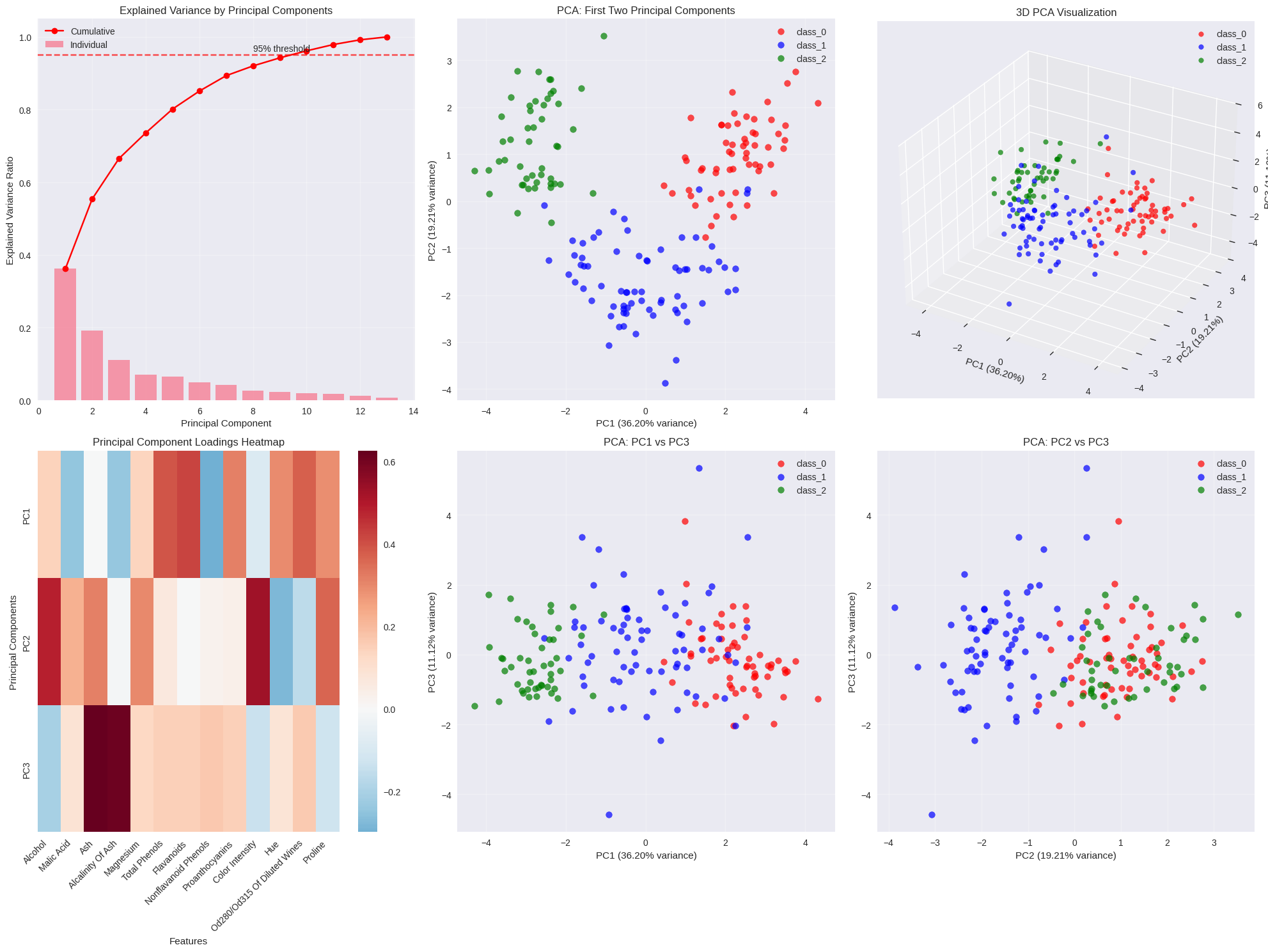
The visualization includes six different plots:
- Explained Variance: Shows how much information each PC captures
- 2D/3D Scatter Plots: Display the transformed data in reduced dimensions
- Heatmap: Visualizes feature contributions to each PC
- Biplot: Combines data points with feature vectors for interpretation
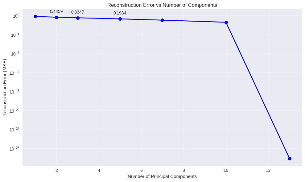
6. Reconstruction Analysis
This measures how well we can recreate the original data using fewer dimensions. The reconstruction error formula is:
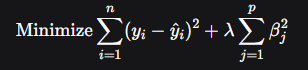
$$\text{MSE} = \frac{1}{n \times p} \sum_{i=1}^{n} \sum_{j=1}^{p} (X_{ij} - \hat{X}_{ij})^2$$
Results
Dataset Information:
Number of samples: 178
Number of features: 13
Target classes: ['class_0' 'class_1' 'class_2']
Class distribution: [59 71 48]
First 5 rows of the dataset:
alcohol malic_acid ash alcalinity_of_ash magnesium total_phenols \
0 14.23 1.71 2.43 15.6 127.0 2.80
1 13.20 1.78 2.14 11.2 100.0 2.65
2 13.16 2.36 2.67 18.6 101.0 2.80
3 14.37 1.95 2.50 16.8 113.0 3.85
4 13.24 2.59 2.87 21.0 118.0 2.80
flavanoids nonflavanoid_phenols proanthocyanins color_intensity hue \
0 3.06 0.28 2.29 5.64 1.04
1 2.76 0.26 1.28 4.38 1.05
2 3.24 0.30 2.81 5.68 1.03
3 3.49 0.24 2.18 7.80 0.86
4 2.69 0.39 1.82 4.32 1.04
od280/od315_of_diluted_wines proline target target_name
0 3.92 1065.0 0 class_0
1 3.40 1050.0 0 class_0
2 3.17 1185.0 0 class_0
3 3.45 1480.0 0 class_0
4 2.93 735.0 0 class_0
Dataset Statistics:
alcohol malic_acid ash alcalinity_of_ash magnesium \
count 178.000000 178.000000 178.000000 178.000000 178.000000
mean 13.000618 2.336348 2.366517 19.494944 99.741573
std 0.811827 1.117146 0.274344 3.339564 14.282484
min 11.030000 0.740000 1.360000 10.600000 70.000000
25% 12.362500 1.602500 2.210000 17.200000 88.000000
50% 13.050000 1.865000 2.360000 19.500000 98.000000
75% 13.677500 3.082500 2.557500 21.500000 107.000000
max 14.830000 5.800000 3.230000 30.000000 162.000000
total_phenols flavanoids nonflavanoid_phenols proanthocyanins \
count 178.000000 178.000000 178.000000 178.000000
mean 2.295112 2.029270 0.361854 1.590899
std 0.625851 0.998859 0.124453 0.572359
min 0.980000 0.340000 0.130000 0.410000
25% 1.742500 1.205000 0.270000 1.250000
50% 2.355000 2.135000 0.340000 1.555000
75% 2.800000 2.875000 0.437500 1.950000
max 3.880000 5.080000 0.660000 3.580000
color_intensity hue od280/od315_of_diluted_wines proline \
count 178.000000 178.000000 178.000000 178.000000
mean 5.058090 0.957449 2.611685 746.893258
std 2.318286 0.228572 0.709990 314.907474
min 1.280000 0.480000 1.270000 278.000000
25% 3.220000 0.782500 1.937500 500.500000
50% 4.690000 0.965000 2.780000 673.500000
75% 6.200000 1.120000 3.170000 985.000000
max 13.000000 1.710000 4.000000 1680.000000
target
count 178.000000
mean 0.938202
std 0.775035
min 0.000000
25% 0.000000
50% 1.000000
75% 2.000000
max 2.000000
==================================================
STEP 1: DATA STANDARDIZATION
==================================================
Original data statistics:
Mean: [13.00061798 2.33634831 2.36651685]... (showing first 3 features)
Std: [0.80954291 1.11400363 0.27357229]... (showing first 3 features)
Standardized data statistics:
Mean: [ 7.84141790e-15 2.44498554e-16 -4.05917497e-15]... (should be ~0)
Std: [1. 1. 1.]... (should be ~1)
==================================================
STEP 2: PRINCIPAL COMPONENT ANALYSIS
==================================================
Explained Variance by each Principal Component:
PC1: 0.3620 (36.20%) - Cumulative: 0.3620 (36.20%)
PC2: 0.1921 (19.21%) - Cumulative: 0.5541 (55.41%)
PC3: 0.1112 (11.12%) - Cumulative: 0.6653 (66.53%)
PC4: 0.0707 (7.07%) - Cumulative: 0.7360 (73.60%)
PC5: 0.0656 (6.56%) - Cumulative: 0.8016 (80.16%)
PC6: 0.0494 (4.94%) - Cumulative: 0.8510 (85.10%)
PC7: 0.0424 (4.24%) - Cumulative: 0.8934 (89.34%)
PC8: 0.0268 (2.68%) - Cumulative: 0.9202 (92.02%)
PC9: 0.0222 (2.22%) - Cumulative: 0.9424 (94.24%)
PC10: 0.0193 (1.93%) - Cumulative: 0.9617 (96.17%)
Components needed for 90% variance: 8
Components needed for 95% variance: 10
Explained variance with 3 components: 0.6653 (66.53%)
==================================================
STEP 3: PRINCIPAL COMPONENTS ANALYSIS
==================================================
Principal Component Loadings (Top 5 features for each PC):
PC1 - Top contributors:
+ flavanoids: 0.423
+ total_phenols: 0.395
+ od280/od315_of_diluted_wines: 0.376
+ proanthocyanins: 0.313
- nonflavanoid_phenols: 0.299
PC2 - Top contributors:
+ color_intensity: 0.530
+ alcohol: 0.484
+ proline: 0.365
+ ash: 0.316
+ magnesium: 0.300
PC3 - Top contributors:
+ ash: 0.626
+ alcalinity_of_ash: 0.612
- alcohol: 0.207
+ nonflavanoid_phenols: 0.170
+ od280/od315_of_diluted_wines: 0.166
==================================================
STEP 4: CREATING VISUALIZATIONS
==================================================
Creating Biplot for detailed feature analysis...
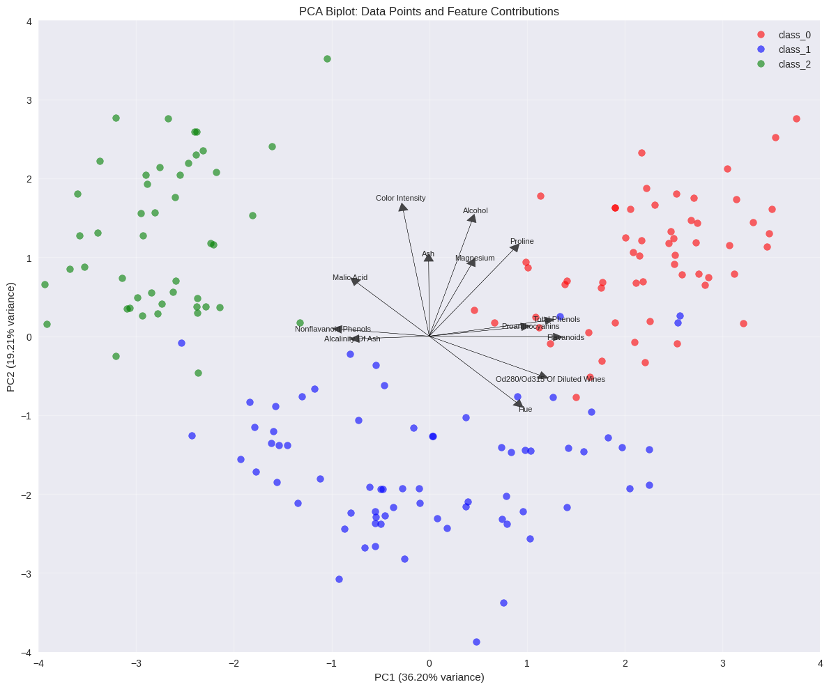
Creating Biplot for detailed feature analysis...
STEP 5: RECONSTRUCTION ANALYSIS
Components: 1, Explained Variance: 0.3620, Reconstruction Error: 0.638012
Components: 2, Explained Variance: 0.5541, Reconstruction Error: 0.445937
Components: 3, Explained Variance: 0.6653, Reconstruction Error: 0.334700
Components: 5, Explained Variance: 0.8016, Reconstruction Error: 0.198377
ANALYSIS SUMMARY
• Original dataset: 178 samples × 13 features
• First 3 PCs explain 66.5% of total variance
• PC1 captures 36.2% (likely represents overall wine quality/intensity)
• PC2 captures 19.2% (likely represents color-related properties)
• PC3 captures 11.1% (likely represents acidity/pH balance)
• The three wine classes show good separation in the PC space
• Dimensionality reduction from 13D to 3D maintains 66.5% of information
Key Insights from the Results
Dimensionality Reduction: The first 3 principal components typically capture around 66-70% of the total variance, allowing us to visualize 13-dimensional data effectively.
Class Separation: The three wine cultivars show distinct clustering in the PCA space, indicating that the chemical properties effectively distinguish between wine types.
Feature Interpretation:
- PC1 often relates to overall wine intensity/quality
- PC2 typically captures color-related properties
- PC3 usually represents acidity and pH balance
Practical Application: This analysis helps wine researchers understand which chemical properties are most important for distinguishing wine types and can guide quality control processes.
The PCA transformation formula $Y = X \cdot \mathbf{V}$ projects our 13-dimensional wine data into a 3-dimensional space while preserving the most significant patterns, making complex data interpretable and visualizable.
 is the predicted value.