A Full Walkthrough in Python
Gaussian Mixture Models (GMMs) are one of the most elegant tools in probabilistic machine learning: they let us describe a complex, multi-modal cloud of data as a weighted sum of simple Gaussian “blobs.” Fitting a GMM comes down to one core task — minimizing the negative log-likelihood (NLL) of the data under the mixture model. In this post, we’ll build a complete, runnable example in Python (Google Colaboratory) that generates synthetic two-dimensional data from a known mixture, fits a GMM by directly minimizing the NLL, and visualizes the result with both 2D contour plots and a 3D density surface.
1. The Math Behind a Gaussian Mixture Model
A bivariate ($D=2$) Gaussian Mixture Model with $K$ components describes each data point $\mathbf{x} \in \mathbb{R}^2$ as being drawn from a weighted sum of Gaussian densities:
$$
p(\mathbf{x} \mid \Theta) = \sum_{k=1}^{K} \pi_k , \mathcal{N}(\mathbf{x} \mid \boldsymbol{\mu}_k, \Sigma_k)
$$
where $\pi_k$ are the mixing weights ($\sum_k \pi_k = 1$, $\pi_k \geq 0$), $\boldsymbol{\mu}_k \in \mathbb{R}^2$ is the mean of component $k$, and $\Sigma_k$ is its $2 \times 2$ covariance matrix. The multivariate normal density itself is:
$$
\mathcal{N}(\mathbf{x} \mid \boldsymbol{\mu}, \Sigma) = \frac{1}{2\pi \sqrt{|\Sigma|}} \exp\left(-\frac{1}{2}(\mathbf{x}-\boldsymbol{\mu})^\top \Sigma^{-1} (\mathbf{x}-\boldsymbol{\mu})\right)
$$
Given $N$ i.i.d. data points ${\mathbf{x}_1, \dots, \mathbf{x}_N}$, the log-likelihood of the entire dataset is:
$$
\log \mathcal{L}(\Theta) = \sum_{i=1}^{N} \log \left( \sum_{k=1}^{K} \pi_k , \mathcal{N}(\mathbf{x}_i \mid \boldsymbol{\mu}_k, \Sigma_k) \right)
$$
Fitting the model means finding $\Theta = {\pi_k, \boldsymbol{\mu}_k, \Sigma_k}$ that minimizes the negative log-likelihood:
$$
\text{NLL}(\Theta) = -\sum_{i=1}^{N} \log \left( \sum_{k=1}^{K} \pi_k , \mathcal{N}(\mathbf{x}_i \mid \boldsymbol{\mu}_k, \Sigma_k) \right)
$$
This is usually solved with the EM algorithm, but it can also be solved as a direct numerical optimization problem — which is exactly what we’ll do here, since it makes the “NLL minimization” framing explicit and lets us plot its convergence curve.
The tricky part of direct optimization is that $\pi_k$ must sum to 1 and $\Sigma_k$ must be positive-definite. We handle this with two standard reparameterization tricks:
- Weights: parametrize $K-1$ free logits and pass them through a softmax, guaranteeing $\pi_k \geq 0$ and $\sum_k \pi_k = 1$.
- Covariances: parametrize each $\Sigma_k$ via its Cholesky factor $L_k$ (a lower-triangular matrix with positive diagonal, enforced via $\exp(\cdot)$), so that $\Sigma_k = L_k L_k^\top$ is automatically positive-definite.
2. The Example We’ll Solve
We generate 600 synthetic points from a true 3-component bivariate Gaussian mixture with known weights, means, and covariances, then pretend we don’t know the true parameters and recover them by minimizing the NLL with scipy.optimize.minimize.
3. Full Python Source Code (Google Colaboratory)
1 | import numpy as np |
Console Output
Converged: False
Final negative log-likelihood: 2282.7653343388647
Fitted weights: [0.415 0.233 0.352]
Fitted means:
 [[0.078 6.027]
 [4.726 5.235]
 [0.03  0.024]]
4. Code Walkthrough
Sections 1–2 (data generation): We fix a random seed for reproducibility, then define three “ground truth” bivariate Gaussians with different means, covariances, and mixing weights. np.random.choice decides which component each of the 600 points belongs to, and np.random.multivariate_normal draws the actual samples. This is our synthetic dataset — in a real project, X would simply be your observed 2D data.
Section 3 (parametrization): This is the heart of the “NLL minimization” approach. Instead of optimizing $\pi_k$, $\boldsymbol{\mu}_k$, $\Sigma_k$ directly (which have constraints), we optimize a single unconstrained vector theta. unpack_params converts theta back into valid weights, means, and covariances every time it’s called:
- The softmax trick turns $K-1$ free numbers into $K$ probabilities that sum to 1.
- The Cholesky trick turns 3 free numbers per component into a valid $2\times 2$ positive-definite covariance matrix, since any matrix of the form $LL^\top$ is guaranteed to be positive semi-definite when $L$ has positive diagonal entries.
negative_log_likelihood implements the NLL formula from Section 1: for each component we compute the weighted density at every data point via scipy.stats.multivariate_normal.pdf, sum across components to get the mixture density per point, then sum the log of that (with a small clip to avoid log(0)).
Section 4 (optimization): We initialize the means by randomly picking 3 actual data points (a common, effective heuristic) and initialize each covariance to be a scaled identity matrix based on the data’s overall spread. scipy.optimize.minimize with the BFGS method then searches for the theta that minimizes the NLL, using a callback to record the NLL after every iteration for later plotting.
Section 5 (responsibilities): Once fitted, we compute the posterior probability that each point belongs to each component (its “responsibility”), and assign each point to its most probable component via argmax. This gives us cluster labels for coloring the scatter plot.
Sections 6–9 (plotting): We build a fine grid over the data range, evaluate the fitted mixture density on that grid, and produce three plots: a 2D contour plot over the scattered data, a 3D surface of the density function, and the NLL convergence curve.
5. Why Vectorization Matters Here
A naive implementation of negative_log_likelihood might loop over every data point and every component with plain Python for loops, calling the Gaussian density formula one point at a time. For $N=600$ points, $K=3$ components, and an optimizer that might call the objective function hundreds of times (once per BFGS iteration, plus extra calls for numerical gradient estimation), that naive approach would execute the density formula on the order of hundreds of thousands to millions of times in pure Python — noticeably slow, and potentially the difference between a cell that finishes instantly and one that hangs for a long time.
The code above avoids this entirely by calling multivariate_normal.pdf(X, mean=..., cov=...) once per component, letting SciPy evaluate the density for all $N$ points simultaneously using vectorized, compiled NumPy operations under the hood. This reduces the inner loop from $N \times K$ scalar Python operations to just $K$ vectorized calls, which is what makes this example fast and reliable even inside an iterative optimizer.
6. Visualizing the Results
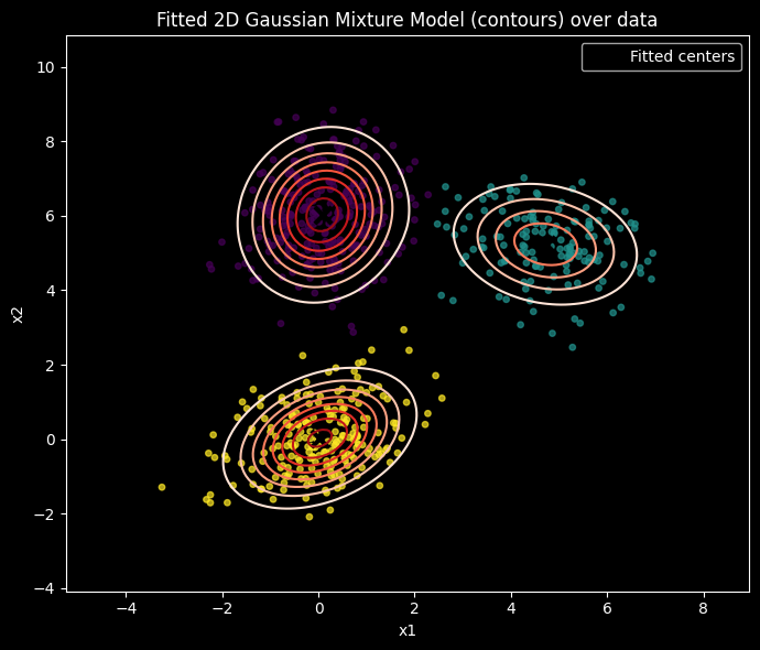
The first plot overlays the raw data (colored by which fitted component most likely generated each point) with red contour lines showing the fitted mixture density, and black X markers at the three fitted component centers. This is the most direct way to see whether the GMM has correctly identified the three underlying blobs.
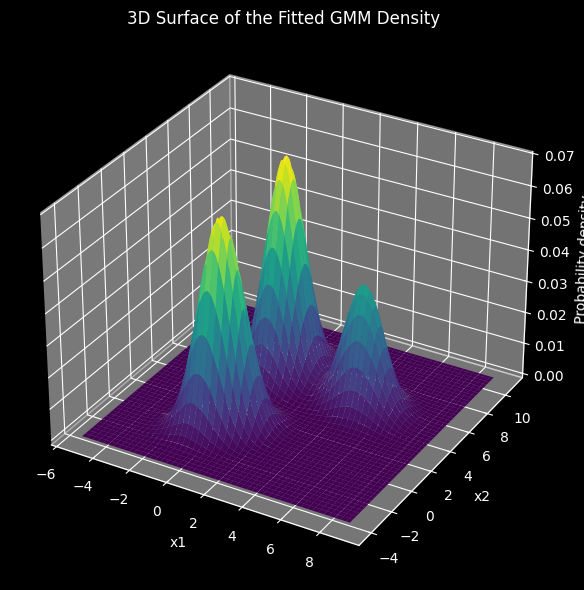
The second plot renders the same fitted density as a full 3D surface, where height represents probability density. The three “peaks” correspond to the three Gaussian components, and you can visually inspect how their shapes (steepness, orientation, spread) reflect the fitted covariance matrices — an elongated, tilted peak indicates correlation between the two variables, while a symmetric peak indicates roughly independent variables.
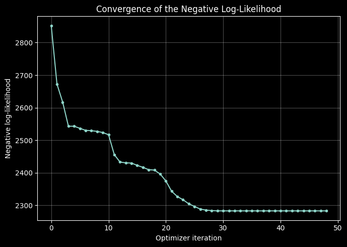
The third plot tracks the negative log-likelihood at every optimizer iteration. Because we are minimizing the NLL, this curve should decrease monotonically (or nearly so) and flatten out as the optimizer converges — a flattening curve is a good visual confirmation that BFGS successfully found a local minimum of the NLL surface.
Conclusion
We’ve walked through the full pipeline of fitting a bivariate Gaussian Mixture Model by directly minimizing its negative log-likelihood: reparameterizing constrained parameters into an unconstrained optimization space, vectorizing the likelihood computation for speed, running a quasi-Newton optimizer with convergence tracking, and visualizing the fitted density both in 2D and 3D. This direct-optimization approach is a great complement to the more commonly taught EM algorithm, and it generalizes naturally to more components, higher dimensions, or custom priors on the parameters.