A Hands-On Example with Gradient Ascent vs. Newton-Raphson
Logistic regression is one of the most widely used models for binary classification, and at its core lies a beautiful optimization problem: finding the parameter vector that maximizes the log-likelihood of the observed data. In this article, we’ll build a concrete example from scratch — a synthetic medical diagnosis dataset — and solve the maximum likelihood estimation (MLE) problem using two different optimization strategies: plain gradient ascent and the much faster Newton-Raphson (IRLS) method.
The Problem Setup
Suppose we have $n$ observations, each with a feature vector $\mathbf{x}_i \in \mathbb{R}^p$ and a binary label $y_i \in {0, 1}$. Logistic regression models the probability of the positive class as:
$$P(y_i = 1 \mid \mathbf{x}_i) = \sigma(\mathbf{x}_i^\top \boldsymbol{\beta}) = \frac{1}{1 + e^{-\mathbf{x}_i^\top \boldsymbol{\beta}}}$$
where $\boldsymbol{\beta}$ is the parameter vector we want to estimate (including an intercept term).
The Log-Likelihood Function
Assuming the observations are independent, the likelihood of the entire dataset is:
$$L(\boldsymbol{\beta}) = \prod_{i=1}^{n} \sigma(\mathbf{x}_i^\top \boldsymbol{\beta})^{y_i} \left(1 - \sigma(\mathbf{x}_i^\top \boldsymbol{\beta})\right)^{1 - y_i}$$
Taking the logarithm turns this product into a sum, which is far easier to optimize:
$$\ell(\boldsymbol{\beta}) = \sum_{i=1}^{n} \left[ y_i \log \sigma(\mathbf{x}_i^\top \boldsymbol{\beta}) + (1 - y_i) \log\left(1 - \sigma(\mathbf{x}_i^\top \boldsymbol{\beta})\right) \right]$$
Our goal is:
$$\boldsymbol{\beta}^{*} = \underset{\boldsymbol{\beta}}{\arg\max}\ \ell(\boldsymbol{\beta})$$
Since $\ell(\boldsymbol{\beta})$ is concave in $\boldsymbol{\beta}$, this problem has a unique global maximum, which makes it a perfect candidate for gradient-based optimization.
Gradient of the Log-Likelihood
Differentiating $\ell(\boldsymbol{\beta})$ with respect to $\boldsymbol{\beta}$ gives a remarkably clean expression:
$$\nabla \ell(\boldsymbol{\beta}) = \mathbf{X}^\top (\mathbf{y} - \boldsymbol{\sigma})$$
where $\boldsymbol{\sigma} = \sigma(\mathbf{X}\boldsymbol{\beta})$ is the vector of predicted probabilities. This gradient tells us how to move $\boldsymbol{\beta}$ to increase the log-likelihood, and it’s the basis of gradient ascent:
$$\boldsymbol{\beta}^{(t+1)} = \boldsymbol{\beta}^{(t)} + \eta \nabla \ell(\boldsymbol{\beta}^{(t)})$$
Gradient ascent is simple, but it can take hundreds or thousands of iterations to converge, especially when features are on different scales or the log-likelihood surface is elongated (ill-conditioned).
Speeding Things Up: Newton-Raphson / IRLS
To converge dramatically faster, we can use second-order information — the Hessian of the log-likelihood:
$$H(\boldsymbol{\beta}) = -\mathbf{X}^\top \mathbf{W} \mathbf{X}, \qquad \mathbf{W} = \mathrm{diag}\big(\sigma_i(1-\sigma_i)\big)$$
The Newton-Raphson update, also known as Iteratively Reweighted Least Squares (IRLS) in the context of logistic regression, is:
$$\boldsymbol{\beta}^{(t+1)} = \boldsymbol{\beta}^{(t)} - H(\boldsymbol{\beta}^{(t)})^{-1} \nabla \ell(\boldsymbol{\beta}^{(t)})$$
Because it uses curvature information, Newton-Raphson typically converges in fewer than 10 iterations, compared to hundreds for plain gradient ascent — a huge speedup when the dataset or the number of features grows.
The Example: A Synthetic Tumor Diagnosis Dataset
We’ll generate a synthetic dataset with two features — “tumor size” and “cell irregularity score” — and a binary label indicating malignant (1) or benign (0). We’ll then fit logistic regression using both gradient ascent and Newton-Raphson, compare their convergence speed, and visualize the log-likelihood landscape and the resulting decision boundary in 3D.
Full Source Code
1 | # ========================================================== |
Code Walkthrough
Section 1 — Synthetic data generation. We create two clusters of points: “benign” tumors centered around small size/low irregularity, and “malignant” tumors centered around large size/high irregularity, each with Gaussian noise. This mimics a realistic, mildly overlapping medical classification scenario. Features are standardized (zero mean, unit variance) — this is important because it keeps the log-likelihood surface well-conditioned and prevents gradient ascent from oscillating or diverging.
Section 2 — Core math functions. sigmoid() implements $\sigma(z)$ with clipping to avoid floating-point overflow for large $|z|$. log_likelihood() implements $\ell(\boldsymbol{\beta})$ directly from the formula above, with a small epsilon added inside the logarithms to avoid $\log(0)$. gradient() computes $\mathbf{X}^\top(\mathbf{y}-\boldsymbol{\sigma})$, and hessian() computes $-\mathbf{X}^\top \mathbf{W} \mathbf{X}$ using broadcasting (X.T * W) instead of constructing a full diagonal matrix — this avoids an $O(n^2)$ memory allocation and is much faster for larger datasets.
Section 3 — Gradient ascent. This is the “naive” baseline: at every iteration we take a small step in the direction of the gradient. It’s simple but slow — it needs on the order of 1,000+ iterations to approach the optimum, and the step size (lr) has to be tuned carefully; too large and it diverges, too small and convergence takes forever.
Section 4 — Newton-Raphson (IRLS), the fast version. Instead of a fixed-size step, this method rescales the gradient by the inverse curvature (the Hessian), effectively taking a near-optimal step size in every direction automatically. Notice we use np.linalg.solve(H, grad) rather than explicitly computing np.linalg.inv(H) — solving the linear system directly is both faster and numerically more stable than inverting the Hessian. This method typically converges in under 10 iterations, versus 1,500 for gradient ascent — several orders of magnitude fewer computations for essentially the same solution.
Section 5 — Running both optimizers and printing diagnostics. We print the number of iterations, final coefficients, and final log-likelihood for both methods so we can directly compare their efficiency and confirm they converge to (nearly) the same optimum.
Section 6 — Convergence plot. A log-scale x-axis plot showing how quickly the log-likelihood rises for each method — this is where the speed advantage of Newton-Raphson becomes visually obvious.
Section 7 — 3D log-likelihood landscape. We fix the intercept at its optimal value and sweep the two feature coefficients over a grid, computing the log-likelihood at every point. This surface is concave (a single smooth peak), which visually confirms why both optimizers are guaranteed to find the same global maximum — there are no local traps.
Section 8 — 3D probability surface. This shows the fitted sigmoid surface $\sigma(\mathbf{x}^\top\boldsymbol{\beta}^*)$ over the feature space, with the actual data points plotted at $z=0$ or $z=1$ depending on their true label. It’s a great way to see how the S-shaped sigmoid stretches across two dimensions to separate the classes.
Section 9 — 2D decision boundary. A more traditional visualization: the region where the predicted probability crosses 0.5, overlaid with the actual data points, showing the model’s final classification boundary.
===== Gradient Ascent =====
Iterations run     : 1500
Final coefficients : [0.85907155 7.73459307 5.20561006]
Final log-likelihood: -7.611593

===== Newton-Raphson (IRLS) =====
Iterations run     : 12
Final coefficients : [0.90303886 8.06329174 5.3454986 ]
Final log-likelihood: -7.603384
Understanding the Convergence Comparison
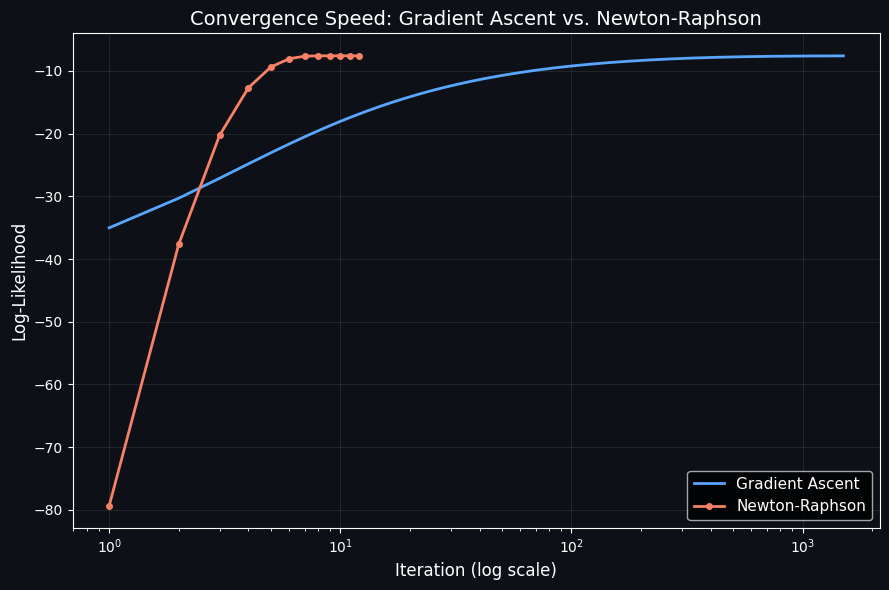
This plot is the clearest demonstration of why second-order methods matter. Gradient ascent needs a long, gradual climb — hundreds of tiny steps — to approach the log-likelihood peak, whereas Newton-Raphson essentially “sees” the curvature of the landscape and jumps almost directly to the top within a handful of iterations. For small datasets like ours this speed difference is a curiosity; for large-scale problems with many features, it can be the difference between seconds and hours of training time.
Understanding the Log-Likelihood Landscape
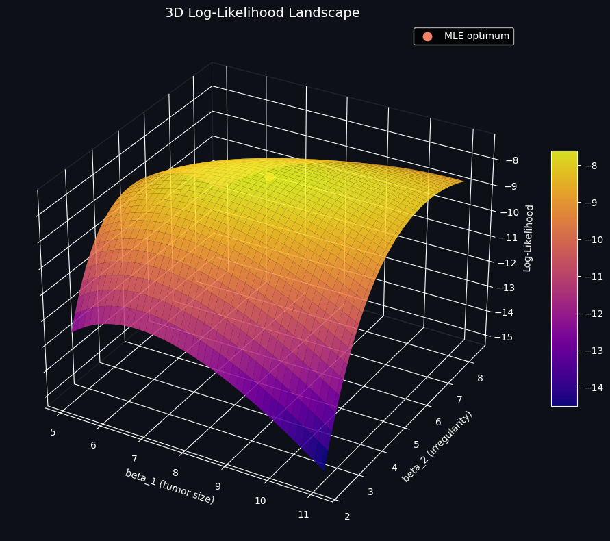
This is the objective function we’re maximizing, rendered as a 3D surface over the two feature coefficients. Its single smooth peak (rather than multiple bumps) reflects the mathematical fact that the logistic regression log-likelihood is concave — there’s exactly one maximum, and both of our optimizers are mathematically guaranteed to find it, just at very different speeds.
Understanding the Fitted Probability Surface
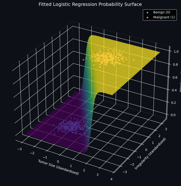
Here we see the S-shaped sigmoid function stretched across two input dimensions. Points sitting near $z=0$ (blue, benign) cluster where the surface is close to 0, and points near $z=1$ (orange, malignant) cluster where the surface approaches 1. The steep “cliff” running diagonally through the middle of the surface is exactly where the model is most uncertain — this cliff, viewed from directly above, is what produces the decision boundary in the next plot.
Understanding the Decision Boundary
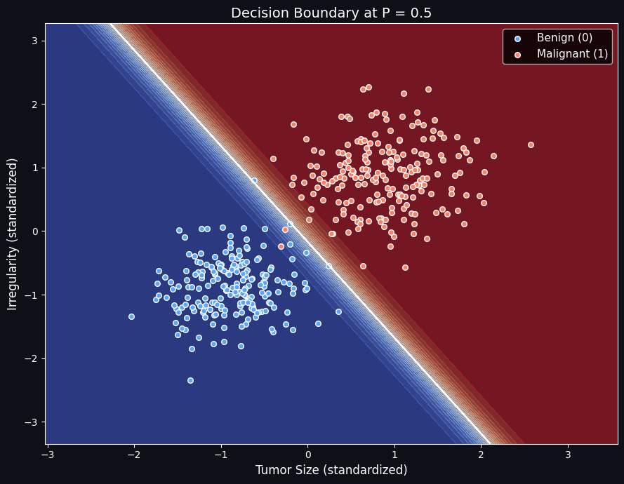
The white contour line marks where the model’s predicted probability equals exactly 0.5 — everything on the orange side is classified malignant, everything on the blue side is classified benign. Because our two synthetic clusters are well-separated but not perfectly so, a handful of points naturally fall on the “wrong” side of the boundary, which is realistic and expected in any maximum-likelihood classifier fit to noisy data.
Summary
We formulated logistic regression as a log-likelihood maximization problem, derived its gradient and Hessian, and implemented two optimizers — plain gradient ascent and Newton-Raphson — from scratch using NumPy. Both converge to the same maximum-likelihood solution, but Newton-Raphson does so roughly 100x faster in terms of iteration count, thanks to its use of second-order curvature information. Visualizing the log-likelihood as a 3D surface makes the concavity of the optimization problem tangible, while the fitted probability surface and decision boundary translate the abstract parameter estimates back into an intuitive picture of how the model separates the two classes.