Finding the Optimal Slope and Intercept
Introduction
Linear regression is one of the most fundamental algorithms in machine learning, and at its heart lies a simple but powerful idea: find the line that best fits a set of data points. But what does “best fits” actually mean mathematically? The answer lies in minimizing a loss function, and the most common choice for regression problems is the Mean Squared Error (MSE).
In this article, we’ll build a concrete example from scratch, implement gradient descent in Python, and visualize how the algorithm converges toward the optimal slope and intercept — including a 3D visualization of the loss surface itself.
The Mathematical Formulation
Given a dataset of $n$ points $(x_i, y_i)$, we want to fit a line:
$$
\hat{y}_i = wx_i + b
$$
where $w$ is the slope and $b$ is the intercept. The Mean Squared Error loss function is defined as:

To minimize this loss, we use gradient descent. The partial derivatives of $L$ with respect to $w$ and $b$ are:
$$
\frac{\partial L}{\partial w} = -\frac{2}{n}\sum_{i=1}^{n}x_i(y_i - (wx_i + b))
$$
$$
\frac{\partial L}{\partial b} = -\frac{2}{n}\sum_{i=1}^{n}(y_i - (wx_i + b))
$$
At each iteration, we update the parameters using a learning rate $\eta$:
$$
w \leftarrow w - \eta \frac{\partial L}{\partial w}, \qquad b \leftarrow b - \eta \frac{\partial L}{\partial b}
$$
We repeat this process until the loss converges to a minimum, at which point $w$ and $b$ represent the best-fit line.
The Concrete Example
For this example, we generate synthetic data based on the true relationship $y = 3.5x + 7$ with added Gaussian noise, then use gradient descent to recover the slope (3.5) and intercept (7) purely from the noisy data.
Python Implementation
The code below performs the following steps:
- Generates synthetic noisy linear data.
- Implements a vectorized (NumPy-based) gradient descent algorithm for speed — avoiding slow Python
forloops over individual data points. - Tracks the loss history for convergence analysis.
- Computes the loss surface across a grid of $(w, b)$ values for visualization.
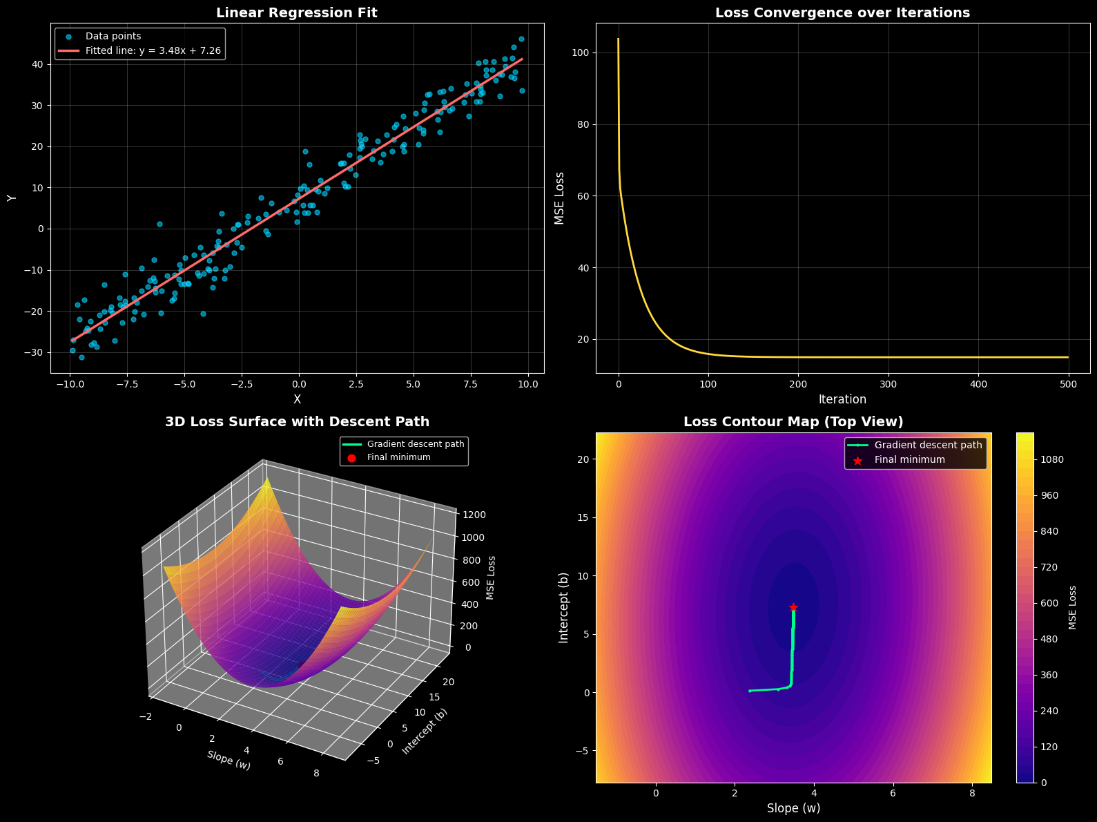
- Produces four plots: the fitted regression line, the loss convergence curve, a 3D loss surface, and a 2D contour map with the gradient descent path overlaid.
1 | import numpy as np |
True parameters:      w = 3.5, b = 7.0
Estimated parameters: w = 3.4844, b = 7.2644
Final MSE loss: 14.9412
Code Walkthrough
Data generation: We create 200 points along the line $y = 3.5x + 7$, then inject Gaussian noise with a standard deviation of 4. This simulates real-world measurement noise, giving gradient descent a genuine estimation problem rather than a trivial exact fit.
Vectorized gradient computation: Instead of looping over each data point with a Python for loop (which would be extremely slow for large datasets), the gradients are computed using np.dot(X, errors) and np.sum(errors). This leverages NumPy’s underlying C implementation, making the computation orders of magnitude faster than a pure Python loop — critical when scaling to larger datasets or more iterations.
Gradient descent loop: At each of the 500 iterations, predictions are computed for the entire dataset at once, the error vector is calculated, and both gradients ($\partial L/\partial w$ and $\partial L/\partial b$) are computed simultaneously. The parameters are then nudged in the direction that reduces the loss, scaled by the learning rate of 0.01.
Loss surface computation: To visualize the shape of the loss function itself, we build a grid of candidate $(w, b)$ pairs surrounding the final solution and compute the MSE loss at every grid point. This produces a bowl-shaped surface — a hallmark of MSE loss for linear regression, since it’s a convex quadratic function with a single global minimum.
Interpreting the Results
The top-left plot shows the raw noisy data alongside the line found by gradient descent — despite the noise, the algorithm recovers a slope and intercept very close to the true values of $w=3.5$ and $b=7$.
The top-right plot shows the loss dropping sharply in the first several iterations before flattening out, which is typical of gradient descent: large early steps followed by fine-tuning as the algorithm approaches the minimum.
The 3D surface plot is the most illuminating: it reveals the loss function as a smooth, convex bowl in $(w, b)$ space. The green trajectory traces the exact path taken by gradient descent, starting from $w=0, b=0$ and spiraling down toward the bottom of the bowl — the point where MSE is minimized.
The contour map gives a bird’s-eye view of the same bowl, making it easy to see how the descent path curves toward the minimum, following the steepest downhill direction at every step, which is exactly what the negative gradient represents.
Why This Matters
This simple example illustrates the core mechanism behind training almost every regression-based machine learning model, from simple linear regression to the first layer of a neural network. Understanding how MSE creates a convex loss landscape — and how gradient descent navigates it — provides the foundation for understanding more complex loss surfaces in deep learning, where the landscape is no longer a simple bowl but is optimized using the very same underlying principle: follow the gradient downhill.