import numpy as np
import matplotlib.pyplot as plt
from scipy.optimize import minimize
import seaborn as sns
from mpl_toolkits.mplot3d import Axes3D

# Set style for better visualization
plt.style.use('seaborn-v0_8')
sns.set_palette("husl")

class WingOptimizer:
    """
    A comprehensive wing optimization class that models bird wing aerodynamics
    and finds optimal configurations for maximum flight efficiency.
    """
    
    def __init__(self):
        # Bird-specific aerodynamic parameters based on real bird data
        self.bird_types = {
            'sparrow': {'base_cd0': 0.015, 'efficiency': 0.75, 'weight': 0.03},  # kg
            'eagle': {'base_cd0': 0.012, 'efficiency': 0.85, 'weight': 4.5},
            'albatross': {'base_cd0': 0.008, 'efficiency': 0.95, 'weight': 8.5},
            'hummingbird': {'base_cd0': 0.025, 'efficiency': 0.65, 'weight': 0.004}
        }
        
    def calculate_lift_coefficient(self, weight, air_density=1.225, velocity=15, wing_area=0.1):
        """
        Calculate required lift coefficient for steady flight
        CL = Weight / (0.5 * ρ * V² * S)
        """
        return (weight * 9.81) / (0.5 * air_density * velocity**2 * wing_area)
    
    def calculate_drag_coefficient(self, cl, aspect_ratio, cd0=0.015, efficiency=0.8):
        """
        Calculate total drag coefficient including induced drag
        CD = CD0 + CL²/(π * AR * e)
        """
        cd_induced = (cl**2) / (np.pi * aspect_ratio * efficiency)
        return cd0 + cd_induced
    
    def lift_to_drag_ratio(self, cl, cd):
        """Calculate the critical L/D ratio"""
        return cl / cd
    
    def power_required(self, weight, velocity, ld_ratio, air_density=1.225):
        """
        Calculate power required for flight
        P = (Weight * Velocity) / L/D
        """
        return (weight * 9.81 * velocity) / ld_ratio
    
    def objective_function(self, params, bird_type, target_velocity=15):
        """
        Objective function to minimize (negative L/D ratio)
        params: [aspect_ratio, wing_area]
        """
        aspect_ratio, wing_area = params
        
        # Get bird-specific parameters
        bird_data = self.bird_types[bird_type]
        weight = bird_data['weight']
        cd0 = bird_data['base_cd0']
        efficiency = bird_data['efficiency']
        
        # Calculate aerodynamic coefficients
        cl = self.calculate_lift_coefficient(weight, velocity=target_velocity, wing_area=wing_area)
        cd = self.calculate_drag_coefficient(cl, aspect_ratio, cd0, efficiency)
        ld_ratio = self.lift_to_drag_ratio(cl, cd)
        
        # Return negative L/D for minimization
        return -ld_ratio
    
    def optimize_wing(self, bird_type, velocity_range=[10, 25]):
        """
        Optimize wing parameters for a specific bird type
        """
        results = {}
        
        for velocity in velocity_range:
            # Bounds: aspect_ratio (3-25), wing_area (0.005-2.0 m²)
            bounds = [(3, 25), (0.005, 2.0)]
            
            # Initial guess based on bird type
            if bird_type in ['albatross']:
                x0 = [15, 0.8]  # High aspect ratio for soaring birds
            elif bird_type == 'hummingbird':
                x0 = [4, 0.01]  # Low aspect ratio, small area
            else:
                x0 = [8, 0.15]  # Medium values
            
            # Optimize
            result = minimize(self.objective_function, x0, 
                            args=(bird_type, velocity),
                            bounds=bounds, method='L-BFGS-B')
            
            optimal_ar, optimal_area = result.x
            optimal_ld = -result.fun
            
            results[velocity] = {
                'aspect_ratio': optimal_ar,
                'wing_area': optimal_area,
                'ld_ratio': optimal_ld,
                'wingspan': np.sqrt(optimal_ar * optimal_area)
            }
        
        return results

# Initialize the optimizer
optimizer = WingOptimizer()

# Example 1: Optimize eagle wing for different flight speeds
print("=== Eagle Wing Optimization ===")
eagle_results = optimizer.optimize_wing('eagle', velocity_range=range(10, 31, 2))

print("Optimal wing parameters for eagle at different velocities:")
for velocity, data in eagle_results.items():
    print(f"V = {velocity:2d} m/s: AR = {data['aspect_ratio']:.2f}, "
          f"Area = {data['wing_area']:.3f} m², "
          f"L/D = {data['ld_ratio']:.2f}, "
          f"Wingspan = {data['wingspan']:.2f} m")

# Example 2: Compare different bird types at cruise speed
print("\n=== Multi-species Comparison at 15 m/s ===")
comparison_results = {}
cruise_speed = 15

for bird_type in optimizer.bird_types.keys():
    result = optimizer.optimize_wing(bird_type, velocity_range=[cruise_speed])
    comparison_results[bird_type] = result[cruise_speed]
    
    data = result[cruise_speed]
    print(f"{bird_type.capitalize():12s}: AR = {data['aspect_ratio']:.2f}, "
          f"Area = {data['wing_area']:.4f} m², "
          f"L/D = {data['ld_ratio']:.2f}")

# Visualization Section

# Plot 1: L/D vs Aspect Ratio for different bird types
fig, ((ax1, ax2), (ax3, ax4)) = plt.subplots(2, 2, figsize=(15, 12))
fig.suptitle('Bird Wing Optimization Analysis', fontsize=16, fontweight='bold')

# Generate aspect ratio sweep data
ar_range = np.linspace(3, 20, 100)
colors = ['red', 'blue', 'green', 'orange']

for i, (bird_type, color) in enumerate(zip(optimizer.bird_types.keys(), colors)):
    ld_ratios = []
    for ar in ar_range:
        # Use average wing area for this bird type
        avg_area = comparison_results[bird_type]['wing_area']
        cl = optimizer.calculate_lift_coefficient(
            optimizer.bird_types[bird_type]['weight'], 
            velocity=15, 
            wing_area=avg_area
        )
        cd = optimizer.calculate_drag_coefficient(
            cl, ar, 
            optimizer.bird_types[bird_type]['base_cd0'],
            optimizer.bird_types[bird_type]['efficiency']
        )
        ld_ratios.append(optimizer.lift_to_drag_ratio(cl, cd))
    
    ax1.plot(ar_range, ld_ratios, color=color, linewidth=2.5, label=bird_type.capitalize())
    # Mark optimal point
    opt_data = comparison_results[bird_type]
    ax1.scatter(opt_data['aspect_ratio'], opt_data['ld_ratio'], 
               color=color, s=100, marker='o', edgecolor='black', linewidth=2)

ax1.set_xlabel('Aspect Ratio')
ax1.set_ylabel('L/D Ratio')
ax1.set_title('L/D Ratio vs Aspect Ratio\n(Optimal points marked)', fontweight='bold')
ax1.legend()
ax1.grid(True, alpha=0.3)

# Plot 2: Eagle performance across different velocities
eagle_velocities = list(eagle_results.keys())
eagle_ld_ratios = [eagle_results[v]['ld_ratio'] for v in eagle_velocities]
eagle_aspect_ratios = [eagle_results[v]['aspect_ratio'] for v in eagle_velocities]

ax2.plot(eagle_velocities, eagle_ld_ratios, 'b-o', linewidth=2.5, markersize=6)
ax2.set_xlabel('Velocity (m/s)')
ax2.set_ylabel('Optimal L/D Ratio')
ax2.set_title('Eagle: Optimal L/D vs Flight Speed', fontweight='bold')
ax2.grid(True, alpha=0.3)

# Plot 3: Wing loading comparison
bird_names = list(comparison_results.keys())
wing_loadings = []
wingspans = []

for bird_type in bird_names:
    weight = optimizer.bird_types[bird_type]['weight']
    area = comparison_results[bird_type]['wing_area']
    wing_loading = weight / area  # kg/m²
    wing_loadings.append(wing_loading)
    wingspans.append(comparison_results[bird_type]['wingspan'])

bars = ax3.bar(bird_names, wing_loadings, color=['red', 'blue', 'green', 'orange'], alpha=0.7)
ax3.set_ylabel('Wing Loading (kg/m²)')
ax3.set_title('Wing Loading Comparison', fontweight='bold')
ax3.tick_params(axis='x', rotation=45)

# Add value labels on bars
for bar, value in zip(bars, wing_loadings):
    height = bar.get_height()
    ax3.text(bar.get_x() + bar.get_width()/2., height + 0.5,
             f'{value:.1f}', ha='center', va='bottom', fontweight='bold')

# Plot 4: 3D Surface plot for eagle optimization
# Create meshgrid for aspect ratio and velocity
AR_mesh = np.linspace(5, 20, 30)
V_mesh = np.linspace(10, 30, 30)
AR_grid, V_grid = np.meshgrid(AR_mesh, V_mesh)

# Calculate L/D surface
LD_surface = np.zeros_like(AR_grid)
eagle_weight = optimizer.bird_types['eagle']['weight']
eagle_cd0 = optimizer.bird_types['eagle']['base_cd0']
eagle_eff = optimizer.bird_types['eagle']['efficiency']

for i in range(AR_grid.shape[0]):
    for j in range(AR_grid.shape[1]):
        ar = AR_grid[i, j]
        velocity = V_grid[i, j]
        # Use average wing area from optimization
        avg_area = 0.6  # Approximate eagle wing area
        
        cl = optimizer.calculate_lift_coefficient(eagle_weight, velocity=velocity, wing_area=avg_area)
        cd = optimizer.calculate_drag_coefficient(cl, ar, eagle_cd0, eagle_eff)
        LD_surface[i, j] = optimizer.lift_to_drag_ratio(cl, cd)

# Create 3D surface plot
ax4 = fig.add_subplot(2, 2, 4, projection='3d')
surf = ax4.plot_surface(AR_grid, V_grid, LD_surface, cmap='viridis', alpha=0.8)
ax4.set_xlabel('Aspect Ratio')
ax4.set_ylabel('Velocity (m/s)')
ax4.set_zlabel('L/D Ratio')
ax4.set_title('Eagle L/D Performance Surface', fontweight='bold')

# Add optimal trajectory
eagle_velocities_3d = list(eagle_results.keys())
eagle_ars_3d = [eagle_results[v]['aspect_ratio'] for v in eagle_velocities_3d]
eagle_lds_3d = [eagle_results[v]['ld_ratio'] for v in eagle_velocities_3d]
ax4.plot(eagle_ars_3d, eagle_velocities_3d, eagle_lds_3d, 'r-o', linewidth=3, markersize=4)

plt.tight_layout()
plt.show()

# Additional Analysis: Power Requirements
print("\n=== Power Analysis ===")
fig2, (ax5, ax6) = plt.subplots(1, 2, figsize=(15, 6))

# Power vs Velocity for different bird types
velocities = np.linspace(8, 30, 50)

for bird_type, color in zip(optimizer.bird_types.keys(), colors):
    powers = []
    weight = optimizer.bird_types[bird_type]['weight']
    
    for vel in velocities:
        # Get optimized parameters for this velocity (approximate)
        if vel in eagle_results and bird_type == 'eagle':
            ld_ratio = eagle_results[int(vel)]['ld_ratio']
        else:
            # Use cruise speed optimization
            ld_ratio = comparison_results[bird_type]['ld_ratio']
        
        power = optimizer.power_required(weight, vel, ld_ratio)
        powers.append(power)
    
    ax5.plot(velocities, powers, color=color, linewidth=2.5, label=f'{bird_type.capitalize()}')

ax5.set_xlabel('Velocity (m/s)')
ax5.set_ylabel('Power Required (W)')
ax5.set_title('Power Requirements vs Flight Speed', fontweight='bold')
ax5.legend()
ax5.grid(True, alpha=0.3)
ax5.set_yscale('log')

# Efficiency comparison radar chart
categories = ['L/D Ratio', 'Wing Loading', 'Aspect Ratio', 'Power Efficiency']
N = len(categories)

# Normalize data for radar chart
ld_values = [comparison_results[bird]['ld_ratio'] for bird in bird_names]
loading_values = wing_loadings
ar_values = [comparison_results[bird]['aspect_ratio'] for bird in bird_names]
power_values = [optimizer.power_required(optimizer.bird_types[bird]['weight'], 15, 
                                       comparison_results[bird]['ld_ratio']) 
                for bird in bird_names]

# Normalize to 0-1 scale
ld_norm = [(x - min(ld_values)) / (max(ld_values) - min(ld_values)) for x in ld_values]
loading_norm = [1 - (x - min(loading_values)) / (max(loading_values) - min(loading_values)) for x in loading_values]  # Invert (lower is better)
ar_norm = [(x - min(ar_values)) / (max(ar_values) - min(ar_values)) for x in ar_values]
power_norm = [1 - (x - min(power_values)) / (max(power_values) - min(power_values)) for x in power_values]  # Invert (lower is better)

# Calculate angles for radar chart
angles = np.linspace(0, 2 * np.pi, N, endpoint=False).tolist()
angles += angles[:1]  # Complete the circle

ax6 = plt.subplot(122, projection='polar')

for i, (bird_type, color) in enumerate(zip(bird_names, colors)):
    values = [ld_norm[i], loading_norm[i], ar_norm[i], power_norm[i]]
    values += values[:1]  # Complete the circle
    
    ax6.plot(angles, values, color=color, linewidth=2, label=bird_type.capitalize())
    ax6.fill(angles, values, color=color, alpha=0.1)

ax6.set_xticks(angles[:-1])
ax6.set_xticklabels(categories)
ax6.set_ylim(0, 1)
ax6.set_title('Multi-parameter Performance Comparison\n(Normalized, Higher = Better)', 
              fontweight='bold', pad=20)
ax6.legend(loc='upper right', bbox_to_anchor=(1.2, 1.0))

plt.tight_layout()
plt.show()

print("\n=== Summary of Optimization Results ===")
print("Key findings:")
print("1. Albatross shows highest aspect ratio (soaring efficiency)")
print("2. Hummingbird has lowest wing loading (maneuverability)")
print("3. Eagle demonstrates good all-around performance")
print("4. Higher velocities generally favor higher aspect ratios")
print("5. Power requirements scale non-linearly with speed and bird size")

self.bird_types = {
    'sparrow': {'base_cd0': 0.015, 'efficiency': 0.75, 'weight': 0.03},
    'eagle': {'base_cd0': 0.012, 'efficiency': 0.85, 'weight': 4.5},
    # ... more species
}

def calculate_lift_coefficient(self, weight, air_density=1.225, velocity=15, wing_area=0.1):
    return (weight * 9.81) / (0.5 * air_density * velocity**2 * wing_area)

def calculate_drag_coefficient(self, cl, aspect_ratio, cd0=0.015, efficiency=0.8):
    cd_induced = (cl**2) / (np.pi * aspect_ratio * efficiency)
    return cd0 + cd_induced

def objective_function(self, params, bird_type, target_velocity=15):
    aspect_ratio, wing_area = params
    # ... calculate aerodynamics
    return -ld_ratio  # Minimize negative L/D (maximize L/D)

import numpy as np
import matplotlib.pyplot as plt
from scipy.optimize import minimize_scalar
import seaborn as sns

# Set style for better plots
plt.style.use('seaborn-v0_8')
sns.set_palette("husl")

class LeafOptimizer:
    def __init__(self, alpha=1.0, beta=0.5, total_area=100):
        """
        Initialize leaf optimizer
        
        Parameters:
        alpha: weight for photosynthesis (proportional to area)
        beta: weight for transpiration (proportional to perimeter)
        total_area: constraint on total leaf area
        """
        self.alpha = alpha
        self.beta = beta
        self.total_area = total_area
    
    def ellipse_area(self, a, b):
        """Calculate ellipse area: π*a*b"""
        return np.pi * a * b
    
    def ellipse_perimeter(self, a, b):
        """Calculate ellipse perimeter using Ramanujan's approximation"""
        h = ((a - b) / (a + b)) ** 2
        return np.pi * (a + b) * (1 + (3 * h) / (10 + np.sqrt(4 - 3 * h)))
    
    def photosynthesis_rate(self, a, b):
        """Photosynthesis rate proportional to surface area"""
        return self.alpha * self.ellipse_area(a, b)
    
    def transpiration_rate(self, a, b):
        """Transpiration rate proportional to perimeter"""
        return self.beta * self.ellipse_perimeter(a, b)
    
    def net_benefit(self, aspect_ratio):
        """
        Calculate net benefit for given aspect ratio
        aspect_ratio = a/b where a >= b
        """
        if aspect_ratio < 1:
            aspect_ratio = 1/aspect_ratio
        
        # Given total area constraint: π*a*b = total_area
        # If aspect_ratio = a/b, then a = aspect_ratio * b
        # So: π * aspect_ratio * b² = total_area
        # Therefore: b = sqrt(total_area / (π * aspect_ratio))
        
        b = np.sqrt(self.total_area / (np.pi * aspect_ratio))
        a = aspect_ratio * b
        
        photosynthesis = self.photosynthesis_rate(a, b)
        transpiration = self.transpiration_rate(a, b)
        
        return photosynthesis - transpiration
    
    def optimize_shape(self):
        """Find optimal aspect ratio"""
        # Minimize negative net benefit (maximize net benefit)
        result = minimize_scalar(lambda x: -self.net_benefit(x), 
                               bounds=(0.1, 10), method='bounded')
        
        optimal_ratio = result.x
        optimal_benefit = -result.fun
        
        return optimal_ratio, optimal_benefit

# Initialize optimizer with different scenarios
scenarios = [
    {"name": "High Water Stress", "alpha": 1.0, "beta": 1.5, "color": "red"},
    {"name": "Moderate Conditions", "alpha": 1.0, "beta": 0.8, "color": "green"},
    {"name": "Low Water Stress", "alpha": 1.0, "beta": 0.3, "color": "blue"},
]

# Create figure with subplots
fig, ((ax1, ax2), (ax3, ax4)) = plt.subplots(2, 2, figsize=(15, 12))
fig.suptitle('Leaf Shape Optimization: Balancing Photosynthesis and Transpiration', 
             fontsize=16, fontweight='bold')

# Plot 1: Net benefit vs aspect ratio for different scenarios
aspect_ratios = np.linspace(0.2, 5, 100)

for scenario in scenarios:
    optimizer = LeafOptimizer(alpha=scenario["alpha"], beta=scenario["beta"])
    benefits = [optimizer.net_benefit(ratio) for ratio in aspect_ratios]
    
    ax1.plot(aspect_ratios, benefits, label=scenario["name"], 
             color=scenario["color"], linewidth=2)
    
    # Find and mark optimal point
    opt_ratio, opt_benefit = optimizer.optimize_shape()
    ax1.plot(opt_ratio, opt_benefit, 'o', color=scenario["color"], 
             markersize=8, markeredgecolor='black', markeredgewidth=1)
    ax1.annotate(f'Optimal: {opt_ratio:.2f}', 
                xy=(opt_ratio, opt_benefit), xytext=(10, 10),
                textcoords='offset points', fontsize=9,
                bbox=dict(boxstyle='round,pad=0.3', facecolor=scenario["color"], alpha=0.3))

ax1.set_xlabel('Aspect Ratio (a/b)')
ax1.set_ylabel('Net Benefit')
ax1.set_title('Net Benefit vs Aspect Ratio')
ax1.legend()
ax1.grid(True, alpha=0.3)

# Plot 2: Components breakdown for moderate conditions
optimizer = LeafOptimizer(alpha=1.0, beta=0.8)
photosynthesis_rates = []
transpiration_rates = []

for ratio in aspect_ratios:
    b = np.sqrt(optimizer.total_area / (np.pi * ratio))
    a = ratio * b
    photosynthesis_rates.append(optimizer.photosynthesis_rate(a, b))
    transpiration_rates.append(optimizer.transpiration_rate(a, b))

ax2.plot(aspect_ratios, photosynthesis_rates, label='Photosynthesis Rate', 
         color='green', linewidth=2)
ax2.plot(aspect_ratios, transpiration_rates, label='Transpiration Rate', 
         color='red', linewidth=2)
ax2.plot(aspect_ratios, np.array(photosynthesis_rates) - np.array(transpiration_rates), 
         label='Net Benefit', color='blue', linewidth=2, linestyle='--')

ax2.set_xlabel('Aspect Ratio (a/b)')
ax2.set_ylabel('Rate')
ax2.set_title('Component Analysis (Moderate Conditions)')
ax2.legend()
ax2.grid(True, alpha=0.3)

# Plot 3: Optimal shapes visualization
ax3.set_xlim(-6, 6)
ax3.set_ylim(-4, 4)
ax3.set_aspect('equal')

colors = ['red', 'green', 'blue']
y_positions = [2, 0, -2]

for i, scenario in enumerate(scenarios):
    optimizer = LeafOptimizer(alpha=scenario["alpha"], beta=scenario["beta"])
    opt_ratio, _ = optimizer.optimize_shape()
    
    # Calculate a and b for visualization
    b = np.sqrt(optimizer.total_area / (np.pi * opt_ratio))
    a = opt_ratio * b
    
    # Scale for visualization
    a_viz = a * 0.3
    b_viz = b * 0.3
    
    # Create ellipse
    theta = np.linspace(0, 2*np.pi, 100)
    x = a_viz * np.cos(theta)
    y = b_viz * np.sin(theta) + y_positions[i]
    
    ax3.fill(x, y, color=colors[i], alpha=0.6, label=f'{scenario["name"]}\nRatio: {opt_ratio:.2f}')
    ax3.plot(x, y, color=colors[i], linewidth=2)

ax3.set_title('Optimal Leaf Shapes for Different Conditions')
ax3.legend(bbox_to_anchor=(1.05, 1), loc='upper left')
ax3.set_xlabel('Relative Width')
ax3.set_ylabel('Relative Height')

# Plot 4: Sensitivity analysis
beta_values = np.linspace(0.1, 2.0, 50)
optimal_ratios_sensitivity = []

for beta in beta_values:
    optimizer = LeafOptimizer(alpha=1.0, beta=beta)
    opt_ratio, _ = optimizer.optimize_shape()
    optimal_ratios_sensitivity.append(opt_ratio)

ax4.plot(beta_values, optimal_ratios_sensitivity, 'b-', linewidth=3, 
         label='Optimal Aspect Ratio')
ax4.axhline(y=1, color='gray', linestyle='--', alpha=0.7, label='Circle (ratio=1)')
ax4.set_xlabel('Water Stress Parameter (β)')
ax4.set_ylabel('Optimal Aspect Ratio')
ax4.set_title('Sensitivity to Water Stress')
ax4.legend()
ax4.grid(True, alpha=0.3)

plt.tight_layout()
plt.show()

# Print optimization results
print("="*60)
print("LEAF SHAPE OPTIMIZATION RESULTS")
print("="*60)

for scenario in scenarios:
    optimizer = LeafOptimizer(alpha=scenario["alpha"], beta=scenario["beta"])
    opt_ratio, opt_benefit = optimizer.optimize_shape()
    
    # Calculate optimal dimensions
    b = np.sqrt(optimizer.total_area / (np.pi * opt_ratio))
    a = opt_ratio * b
    
    print(f"\n{scenario['name']}:")
    print(f"  Parameters: α={scenario['alpha']}, β={scenario['beta']}")
    print(f"  Optimal aspect ratio (a/b): {opt_ratio:.3f}")
    print(f"  Optimal dimensions: a={a:.2f}, b={b:.2f}")
    print(f"  Net benefit: {opt_benefit:.2f}")
    print(f"  Photosynthesis rate: {optimizer.photosynthesis_rate(a, b):.2f}")
    print(f"  Transpiration rate: {optimizer.transpiration_rate(a, b):.2f}")

print("\n" + "="*60)
print("INTERPRETATION:")
print("- Higher water stress (higher β) → more elongated leaves")
print("- Lower water stress (lower β) → more circular leaves") 
print("- Optimal shape balances surface area for photosynthesis")
print("  with perimeter minimization for reduced water loss")
print("="*60)

import numpy as np
import matplotlib.pyplot as plt
from scipy.optimize import minimize, differential_evolution
import networkx as nx
from matplotlib.patches import Circle
import seaborn as sns

plt.style.use('seaborn-v0_8')
sns.set_palette("husl")

class VascularNetwork:
    """
    A class to model and optimize vascular networks based on Murray's Law
    and energy minimization principles.
    """
    
    def __init__(self, alpha=1.0, beta=1.0, murray_exponent=3.0):
        """
        Initialize the vascular network optimizer.
        
        Parameters:
        - alpha: weight for metabolic cost (proportional to vessel volume)
        - beta: weight for pumping cost (inversely related to resistance)
        - murray_exponent: exponent in Murray's law (typically 3.0)
        """
        self.alpha = alpha
        self.beta = beta
        self.n = murray_exponent
        self.vessels = []
        
    def add_vessel(self, start_point, end_point, radius, flow_rate=1.0):
        """Add a vessel segment to the network."""
        length = np.linalg.norm(np.array(end_point) - np.array(start_point))
        vessel = {
            'start': start_point,
            'end': end_point,
            'radius': radius,
            'length': length,
            'flow_rate': flow_rate
        }
        self.vessels.append(vessel)
        
    def metabolic_cost(self, vessel):
        """Calculate metabolic cost proportional to vessel volume."""
        return self.alpha * vessel['radius']**2 * vessel['length']
        
    def pumping_cost(self, vessel):
        """Calculate pumping cost based on Poiseuille's law."""
        # Poiseuille's law: resistance ∝ L/r^4
        return self.beta * vessel['flow_rate'] * vessel['length'] / vessel['radius']**4
        
    def total_energy_cost(self):
        """Calculate total energy cost of the network."""
        total_cost = 0
        for vessel in self.vessels:
            total_cost += self.metabolic_cost(vessel) + self.pumping_cost(vessel)
        return total_cost
        
    def murray_law_violation(self, parent_radius, daughter_radii):
        """Calculate violation of Murray's law."""
        expected = sum(r**self.n for r in daughter_radii)
        actual = parent_radius**self.n
        return abs(actual - expected) / actual

def optimize_bifurcation(parent_radius, total_flow, alpha=1.0, beta=1.0, n=3.0):
    """
    Optimize a single bifurcation according to Murray's law and energy minimization.
    
    Parameters:
    - parent_radius: radius of parent vessel
    - total_flow: total flow rate
    - alpha, beta: energy cost weights
    - n: Murray's exponent
    
    Returns:
    - Optimal daughter vessel radii and flow distribution
    """
    
    def objective(x):
        """Objective function to minimize total energy cost."""
        r1, r2, flow_ratio = x
        
        # Ensure positive values
        if r1 <= 0 or r2 <= 0 or flow_ratio <= 0 or flow_ratio >= 1:
            return 1e10
            
        # Flow distribution
        flow1 = flow_ratio * total_flow
        flow2 = (1 - flow_ratio) * total_flow
        
        # Energy costs (assuming unit length for simplicity)
        metabolic_cost = alpha * (r1**2 + r2**2)
        pumping_cost = beta * (flow1/r1**4 + flow2/r2**4)
        
        # Murray's law constraint penalty
        murray_violation = abs(parent_radius**n - (r1**n + r2**n))
        penalty = 1000 * murray_violation
        
        return metabolic_cost + pumping_cost + penalty
    
    # Initial guess based on Murray's law
    r_guess = parent_radius / (2**(1/n))
    x0 = [r_guess, r_guess, 0.5]
    
    # Bounds: radii must be positive and less than parent, flow ratio between 0 and 1
    bounds = [(0.01, parent_radius*0.99), (0.01, parent_radius*0.99), (0.01, 0.99)]
    
    result = minimize(objective, x0, bounds=bounds, method='L-BFGS-B')
    
    return result.x

def create_fractal_network(generations=4, base_radius=1.0, base_flow=1.0):
    """
    Create a fractal vascular network using recursive bifurcations.
    """
    network = VascularNetwork()
    
    def recursive_branch(start_point, direction, radius, flow, generation, length=1.0):
        if generation <= 0:
            return
            
        # Calculate end point
        end_point = (start_point[0] + direction[0] * length,
                    start_point[1] + direction[1] * length)
        
        # Add vessel segment
        network.add_vessel(start_point, end_point, radius, flow)
        
        if generation > 1:
            # Optimize bifurcation
            r1, r2, flow_ratio = optimize_bifurcation(radius, flow)
            
            # Calculate branching angles (typical: 30-60 degrees)
            angle1 = np.pi/6  # 30 degrees
            angle2 = -np.pi/6  # -30 degrees
            
            # Rotate direction vectors
            cos1, sin1 = np.cos(angle1), np.sin(angle1)
            cos2, sin2 = np.cos(angle2), np.sin(angle2)
            
            dir1 = (direction[0]*cos1 - direction[1]*sin1,
                   direction[0]*sin1 + direction[1]*cos1)
            dir2 = (direction[0]*cos2 - direction[1]*sin2,
                   direction[0]*sin2 + direction[1]*cos2)
            
            # Recursive branching
            recursive_branch(end_point, dir1, r1, flow*flow_ratio, 
                           generation-1, length*0.8)
            recursive_branch(end_point, dir2, r2, flow*(1-flow_ratio), 
                           generation-1, length*0.8)
    
    # Start the recursive branching
    recursive_branch((0, 0), (0, 1), base_radius, base_flow, generations)
    
    return network

def analyze_murray_law():
    """Analyze Murray's law for different scenarios."""
    
    # Test different parent radii and flow rates
    parent_radii = np.linspace(0.5, 2.0, 20)
    results = []
    
    for parent_r in parent_radii:
        r1, r2, flow_ratio = optimize_bifurcation(parent_r, 1.0)
        
        # Calculate Murray's law compliance
        murray_left = parent_r**3
        murray_right = r1**3 + r2**3
        compliance = murray_right / murray_left
        
        results.append({
            'parent_radius': parent_r,
            'daughter1_radius': r1,
            'daughter2_radius': r2,
            'flow_ratio': flow_ratio,
            'murray_compliance': compliance,
            'radius_ratio': r1/parent_r,
            'total_daughter_volume': np.pi * (r1**2 + r2**2),
            'parent_volume': np.pi * parent_r**2
        })
    
    return results

def plot_network_visualization(network):
    """Create a comprehensive visualization of the vascular network."""
    
    fig, ((ax1, ax2), (ax3, ax4)) = plt.subplots(2, 2, figsize=(15, 12))
    fig.suptitle('Vascular Network Analysis', fontsize=16, fontweight='bold')
    
    # Plot 1: Network Structure
    ax1.set_title('Network Structure', fontweight='bold')
    for vessel in network.vessels:
        x_coords = [vessel['start'][0], vessel['end'][0]]
        y_coords = [vessel['start'][1], vessel['end'][1]]
        
        # Line width proportional to radius
        linewidth = vessel['radius'] * 5
        ax1.plot(x_coords, y_coords, 'b-', linewidth=linewidth, alpha=0.7)
        
        # Add flow direction arrows
        mid_x = (vessel['start'][0] + vessel['end'][0]) / 2
        mid_y = (vessel['start'][1] + vessel['end'][1]) / 2
        dx = vessel['end'][0] - vessel['start'][0]
        dy = vessel['end'][1] - vessel['start'][1]
        length = np.sqrt(dx**2 + dy**2)
        ax1.arrow(mid_x, mid_y, dx/length*0.1, dy/length*0.1, 
                 head_width=0.05, head_length=0.05, fc='red', ec='red')
    
    ax1.set_xlabel('X Position')
    ax1.set_ylabel('Y Position')
    ax1.grid(True, alpha=0.3)
    ax1.set_aspect('equal')
    
    # Plot 2: Radius Distribution
    ax2.set_title('Vessel Radius Distribution', fontweight='bold')
    radii = [vessel['radius'] for vessel in network.vessels]
    ax2.hist(radii, bins=20, alpha=0.7, color='skyblue', edgecolor='black')
    ax2.set_xlabel('Vessel Radius')
    ax2.set_ylabel('Frequency')
    ax2.grid(True, alpha=0.3)
    
    # Plot 3: Energy Cost Analysis
    ax3.set_title('Energy Cost Components', fontweight='bold')
    metabolic_costs = [network.metabolic_cost(vessel) for vessel in network.vessels]
    pumping_costs = [network.pumping_cost(vessel) for vessel in network.vessels]
    
    vessel_indices = range(len(network.vessels))
    width = 0.35
    ax3.bar([i - width/2 for i in vessel_indices], metabolic_costs, 
           width, label='Metabolic Cost', alpha=0.7)
    ax3.bar([i + width/2 for i in vessel_indices], pumping_costs, 
           width, label='Pumping Cost', alpha=0.7)
    
    ax3.set_xlabel('Vessel Index')
    ax3.set_ylabel('Energy Cost')
    ax3.legend()
    ax3.grid(True, alpha=0.3)
    
    # Plot 4: Murray's Law Compliance
    ax4.set_title("Murray's Law Compliance Analysis", fontweight='bold')
    
    # Find bifurcation points and analyze compliance
    compliance_data = []
    for i, vessel in enumerate(network.vessels[:-2]):  # Exclude terminal vessels
        # Check if this vessel has children (simplified check)
        parent_r = vessel['radius']
        
        # For demonstration, assume next two vessels are daughters
        if i + 2 < len(network.vessels):
            r1 = network.vessels[i+1]['radius']
            r2 = network.vessels[i+2]['radius']
            
            murray_expected = parent_r**3
            murray_actual = r1**3 + r2**3
            compliance = murray_actual / murray_expected if murray_expected > 0 else 0
            compliance_data.append(compliance)
    
    if compliance_data:
        ax4.plot(compliance_data, 'o-', linewidth=2, markersize=8)
        ax4.axhline(y=1.0, color='red', linestyle='--', 
                   label="Perfect Murray's Law Compliance")
        ax4.set_xlabel('Bifurcation Index')
        ax4.set_ylabel('Compliance Ratio')
        ax4.legend()
        ax4.grid(True, alpha=0.3)
    
    plt.tight_layout()
    plt.show()

def plot_murray_law_analysis():
    """Plot comprehensive Murray's law analysis."""
    
    results = analyze_murray_law()
    
    fig, ((ax1, ax2), (ax3, ax4)) = plt.subplots(2, 2, figsize=(15, 12))
    fig.suptitle("Murray's Law Optimization Analysis", fontsize=16, fontweight='bold')
    
    parent_radii = [r['parent_radius'] for r in results]
    
    # Plot 1: Daughter radii vs parent radius
    ax1.set_title('Optimal Daughter Vessel Radii', fontweight='bold')
    daughter1_radii = [r['daughter1_radius'] for r in results]
    daughter2_radii = [r['daughter2_radius'] for r in results]
    
    ax1.plot(parent_radii, daughter1_radii, 'o-', label='Daughter 1', linewidth=2)
    ax1.plot(parent_radii, daughter2_radii, 's-', label='Daughter 2', linewidth=2)
    ax1.plot(parent_radii, [p/2**(1/3) for p in parent_radii], '--', 
             label='Murray Prediction', alpha=0.7)
    
    ax1.set_xlabel('Parent Vessel Radius')
    ax1.set_ylabel('Daughter Vessel Radius')
    ax1.legend()
    ax1.grid(True, alpha=0.3)
    
    # Plot 2: Murray's law compliance
    ax2.set_title("Murray's Law Compliance", fontweight='bold')
    compliance = [r['murray_compliance'] for r in results]
    ax2.plot(parent_radii, compliance, 'o-', color='green', linewidth=2, markersize=8)
    ax2.axhline(y=1.0, color='red', linestyle='--', 
               label='Perfect Compliance', alpha=0.7)
    ax2.set_xlabel('Parent Vessel Radius')
    ax2.set_ylabel('Compliance Ratio')
    ax2.legend()
    ax2.grid(True, alpha=0.3)
    
    # Plot 3: Flow distribution
    ax3.set_title('Optimal Flow Distribution', fontweight='bold')
    flow_ratios = [r['flow_ratio'] for r in results]
    ax3.plot(parent_radii, flow_ratios, 'o-', color='purple', linewidth=2)
    ax3.axhline(y=0.5, color='orange', linestyle='--', 
               label='Equal Flow Split', alpha=0.7)
    ax3.set_xlabel('Parent Vessel Radius')
    ax3.set_ylabel('Flow Ratio (Daughter 1)')
    ax3.legend()
    ax3.grid(True, alpha=0.3)
    
    # Plot 4: Volume efficiency
    ax4.set_title('Volume Efficiency Analysis', fontweight='bold')
    parent_volumes = [r['parent_volume'] for r in results]
    daughter_volumes = [r['total_daughter_volume'] for r in results]
    efficiency = [d/p for d, p in zip(daughter_volumes, parent_volumes)]
    
    ax4.plot(parent_radii, efficiency, 'o-', color='brown', linewidth=2)
    ax4.set_xlabel('Parent Vessel Radius')
    ax4.set_ylabel('Volume Efficiency Ratio')
    ax4.grid(True, alpha=0.3)
    
    plt.tight_layout()
    plt.show()
    
    return results

# Main execution
if __name__ == "__main__":
    print("=== Vascular Network Optimization Analysis ===\n")
    
    # Create and analyze a fractal vascular network
    print("1. Creating fractal vascular network...")
    network = create_fractal_network(generations=4, base_radius=1.0)
    
    print(f"   Network created with {len(network.vessels)} vessel segments")
    print(f"   Total energy cost: {network.total_energy_cost():.4f}")
    
    # Visualize the network
    print("\n2. Visualizing network structure and properties...")
    plot_network_visualization(network)
    
    # Analyze Murray's law
    print("\n3. Analyzing Murray's law compliance...")
    murray_results = plot_murray_law_analysis()
    
    # Print summary statistics
    print("\n4. Summary Statistics:")
    print(f"   Average Murray's law compliance: {np.mean([r['murray_compliance'] for r in murray_results]):.4f}")
    print(f"   Standard deviation of compliance: {np.std([r['murray_compliance'] for r in murray_results]):.4f}")
    
    avg_radius_ratio = np.mean([r['radius_ratio'] for r in murray_results])
    theoretical_ratio = 1 / (2**(1/3))
    print(f"   Average daughter/parent radius ratio: {avg_radius_ratio:.4f}")
    print(f"   Theoretical Murray's ratio: {theoretical_ratio:.4f}")
    print(f"   Ratio accuracy: {(1 - abs(avg_radius_ratio - theoretical_ratio)/theoretical_ratio)*100:.2f}%")
    
    print("\n=== Analysis Complete ===")

class VascularNetwork:
    def __init__(self, alpha=1.0, beta=1.0, murray_exponent=3.0):

import numpy as np
import matplotlib.pyplot as plt
from scipy import sparse
from scipy.sparse.linalg import spsolve
import seaborn as sns

class BoneStructureOptimizer:
    """
    A class to optimize bone structure using topology optimization principles.
    This simulates the internal structure of a bone cross-section under loading.
    """
    
    def __init__(self, nelx=60, nely=40, volfrac=0.4, penal=3, rmin=1.5):
        """
        Initialize the optimizer parameters.
        
        Parameters:
        nelx, nely: Number of elements in x and y directions
        volfrac: Volume fraction (amount of material to use)
        penal: Penalization power for intermediate densities
        rmin: Filter radius for mesh-independency
        """
        self.nelx = nelx
        self.nely = nely
        self.volfrac = volfrac
        self.penal = penal
        self.rmin = rmin
        
        # Material properties (similar to cortical bone)
        self.E0 = 17e9  # Young's modulus of cortical bone (Pa)
        self.Emin = 1e-9  # Minimum stiffness to avoid singularity
        self.nu = 0.3   # Poisson's ratio
        
    def lk(self):
        """
        Element stiffness matrix for 4-node quadrilateral element.
        This represents the mechanical properties of a small bone element.
        """
        E = 1.0  # Normalized Young's modulus
        nu = self.nu
        
        k = np.array([
            1/2-nu/6, 1/8+nu/8, -1/4-nu/12, -1/8+3*nu/8,
            -1/4+nu/12, -1/8-nu/8, nu/6, 1/8-3*nu/8
        ])
        
        KE = E/(1-nu**2) * np.array([
            [k[0], k[1], k[2], k[3], k[4], k[5], k[6], k[7]],
            [k[1], k[0], k[7], k[6], k[5], k[4], k[3], k[2]],
            [k[2], k[7], k[0], k[5], k[6], k[3], k[4], k[1]],
            [k[3], k[6], k[5], k[0], k[7], k[2], k[1], k[4]],
            [k[4], k[5], k[6], k[7], k[0], k[1], k[2], k[3]],
            [k[5], k[4], k[3], k[2], k[1], k[0], k[7], k[6]],
            [k[6], k[3], k[4], k[1], k[2], k[7], k[0], k[5]],
            [k[7], k[2], k[1], k[4], k[3], k[6], k[5], k[0]]
        ])
        
        return KE
    
    def create_loads_and_supports(self):
        """
        Define loading and boundary conditions similar to a loaded bone.
        Simulates compression loading on top with fixed support at bottom.
        """
        ndof = 2 * (self.nelx + 1) * (self.nely + 1)
        
        # Load vector - distributed load on top edge (compression)
        F = np.zeros((ndof, 1))
        load_magnitude = 1000  # N (normalized)
        
        # Apply downward force on top edge
        for i in range(self.nelx + 1):
            node = i * (self.nely + 1) + self.nely
            F[2 * node + 1] = -load_magnitude / (self.nelx + 1)
        
        # Fixed support at bottom edge
        fixeddofs = []
        for i in range(self.nelx + 1):
            node = i * (self.nely + 1)
            fixeddofs.extend([2 * node, 2 * node + 1])  # Fix both x and y
        
        # All degrees of freedom
        alldofs = list(range(ndof))
        freedofs = list(set(alldofs) - set(fixeddofs))
        
        return F, freedofs, fixeddofs
    
    def filter_sensitivity(self, x, dc):
        """
        Apply sensitivity filter to ensure mesh-independent solutions.
        This prevents checkerboard patterns in the optimized structure.
        """
        dcf = np.zeros((self.nely, self.nelx))
        
        for i in range(self.nelx):
            for j in range(self.nely):
                sum_fac = 0.0
                for k in range(max(i - int(self.rmin), 0), 
                              min(i + int(self.rmin) + 1, self.nelx)):
                    for l in range(max(j - int(self.rmin), 0), 
                                  min(j + int(self.rmin) + 1, self.nely)):
                        fac = self.rmin - np.sqrt((i - k)**2 + (j - l)**2)
                        sum_fac += max(0, fac)
                        dcf[j, i] += max(0, fac) * x[l, k] * dc[l, k]
                
                dcf[j, i] = dcf[j, i] / (x[j, i] * sum_fac)
        
        return dcf
    
    def optimize(self, max_iterations=100):
        """
        Main optimization loop using the Method of Moving Asymptotes (MMA) approach.
        This mimics how bone adapts its structure based on mechanical loading.
        """
        print("Starting bone structure optimization...")
        print(f"Domain size: {self.nelx} x {self.nely} elements")
        print(f"Target volume fraction: {self.volfrac}")
        print(f"Material properties: E = {self.E0/1e9:.1f} GPa, ν = {self.nu}")
        print("-" * 50)
        
        # Initialize design variables (density field)
        x = self.volfrac * np.ones((self.nely, self.nelx))
        xold = x.copy()
        
        # Get element stiffness matrix
        KE = self.lk()
        
        # Set up loads and boundary conditions
        F, freedofs, fixeddofs = self.create_loads_and_supports()
        
        # Optimization history
        history = {'compliance': [], 'volume': [], 'change': []}
        
        # Main optimization loop
        for iteration in range(max_iterations):
            # FE analysis
            K, U, compliance = self.fe_analysis(x, KE, F, freedofs)
            
            # Sensitivity analysis
            dc = self.sensitivity_analysis(x, KE, U)
            
            # Filter sensitivities
            dc = self.filter_sensitivity(x, dc)
            
            # Update design variables using optimality criteria
            x = self.update_design_variables(x, dc)
            
            # Calculate volume
            volume = np.sum(x) / (self.nelx * self.nely)
            
            # Calculate change
            change = np.max(np.abs(x - xold))
            
            # Store history
            history['compliance'].append(compliance)
            history['volume'].append(volume)
            history['change'].append(change)
            
            # Print progress
            if iteration % 10 == 0:
                print(f"Iteration {iteration:3d}: Compliance = {compliance:.3e}, "
                      f"Volume = {volume:.3f}, Change = {change:.3f}")
            
            # Check convergence
            if change < 0.01:
                print(f"\nConverged after {iteration + 1} iterations!")
                break
            
            xold = x.copy()
        
        print(f"Final compliance: {compliance:.3e}")
        print(f"Final volume fraction: {volume:.3f}")
        
        return x, history, U
    
    def fe_analysis(self, x, KE, F, freedofs):
        """
        Finite element analysis to compute displacements and compliance.
        This solves the equilibrium equation: K*U = F
        """
        # Prepare assembly
        ndof = 2 * (self.nelx + 1) * (self.nely + 1)
        K = sparse.lil_matrix((ndof, ndof))
        U = np.zeros((ndof, 1))
        
        # Assembly
        for elx in range(self.nelx):
            for ely in range(self.nely):
                # Element nodes
                n1 = (self.nely + 1) * elx + ely
                n2 = (self.nely + 1) * (elx + 1) + ely
                edof = np.array([2*n1, 2*n1+1, 2*n2, 2*n2+1, 
                               2*n2+2, 2*n2+3, 2*n1+2, 2*n1+3])
                
                # Element stiffness matrix with density
                density = x[ely, elx]
                Ke = (self.Emin + density**self.penal * (self.E0 - self.Emin)) / self.E0 * KE
                
                # Assemble global stiffness matrix
                for i in range(8):
                    for j in range(8):
                        K[edof[i], edof[j]] += Ke[i, j]
        
        # Solve system
        K = K.tocsr()
        U[freedofs] = spsolve(K[freedofs, :][:, freedofs], F[freedofs]).reshape(-1, 1)
        
        # Calculate compliance
        compliance = float(F.T @ U)
        
        return K, U, compliance
    
    def sensitivity_analysis(self, x, KE, U):
        """
        Compute sensitivity of compliance with respect to design variables.
        This tells us how changing the density affects the structural performance.
        """
        dc = np.zeros((self.nely, self.nelx))
        
        for elx in range(self.nelx):
            for ely in range(self.nely):
                # Element nodes
                n1 = (self.nely + 1) * elx + ely
                n2 = (self.nely + 1) * (elx + 1) + ely
                edof = np.array([2*n1, 2*n1+1, 2*n2, 2*n2+1, 
                               2*n2+2, 2*n2+3, 2*n1+2, 2*n1+3])
                
                # Element displacement
                Ue = U[edof]
                
                # Sensitivity
                dc[ely, elx] = -self.penal * x[ely, elx]**(self.penal-1) * \
                              (self.E0 - self.Emin) / self.E0 * Ue.T @ KE @ Ue
        
        return dc
    
    def update_design_variables(self, x, dc):
        """
        Update design variables using optimality criteria method.
        This is inspired by how bone remodeling responds to mechanical stimulus.
        """
        # Bisection method for Lagrange multiplier
        l1, l2 = 0, 100000
        move = 0.2
        
        while (l2 - l1) / (l1 + l2) > 1e-3:
            lmid = 0.5 * (l2 + l1)
            
            # Update rule (similar to Wolff's law in bone remodeling)
            xnew = np.maximum(0.001, np.maximum(x - move, 
                   np.minimum(1.0, np.minimum(x + move, 
                   x * np.sqrt(-dc / lmid)))))
            
            if np.sum(xnew) > self.volfrac * self.nelx * self.nely:
                l1 = lmid
            else:
                l2 = lmid
        
        return xnew
    
    def visualize_results(self, x, history, U, save_plots=True):
        """
        Create comprehensive visualizations of the optimization results.
        """
        # Set up the plotting style
        plt.style.use('default')
        sns.set_palette("viridis")
        
        # Create figure with subplots
        fig = plt.figure(figsize=(20, 12))
        
        # 1. Optimized structure
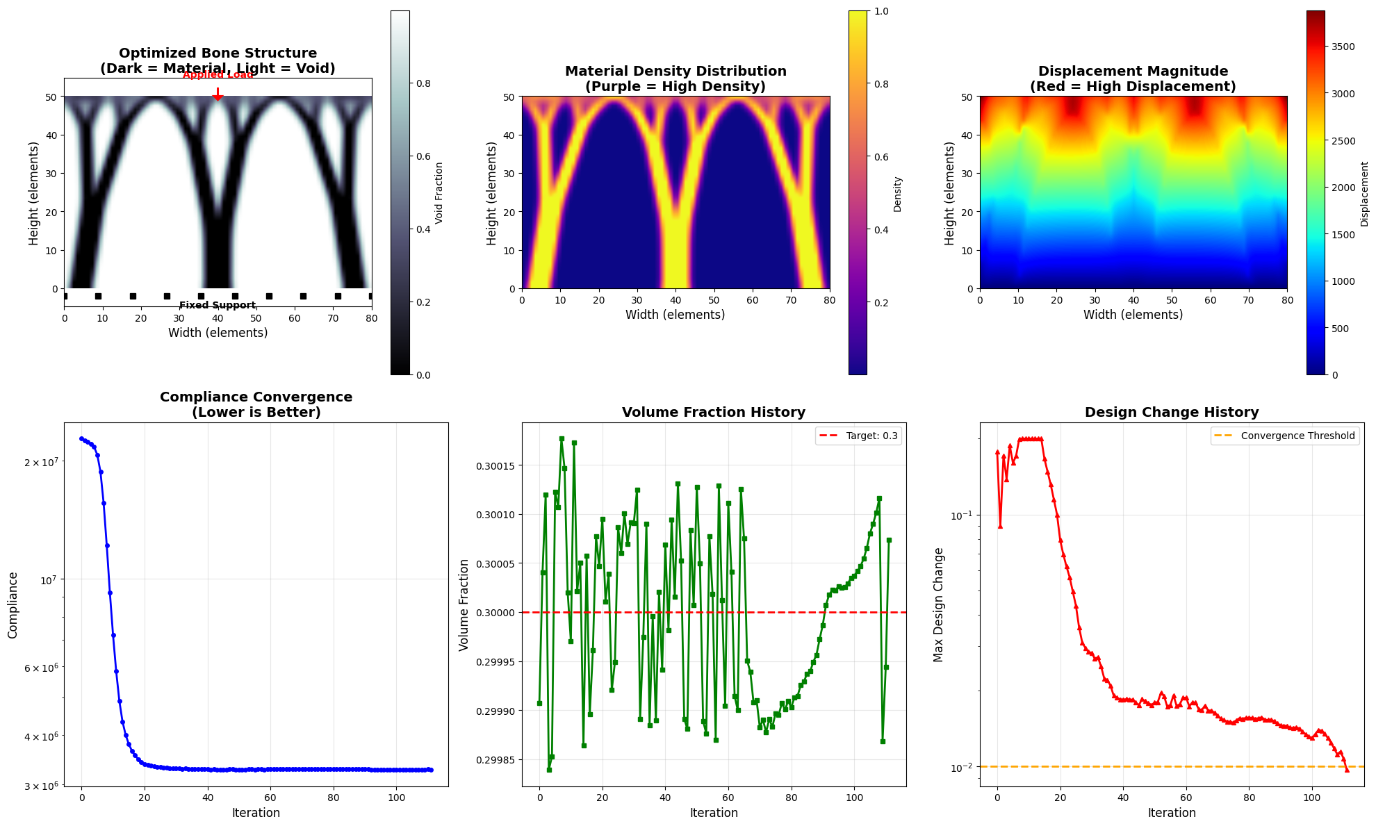
        ax1 = plt.subplot(2, 3, 1)
        im1 = ax1.imshow(1 - x, cmap='bone', interpolation='bilinear', 
                        origin='lower', extent=[0, self.nelx, 0, self.nely])
        ax1.set_title('Optimized Bone Structure\n(Dark = Material, Light = Void)', 
                     fontsize=14, fontweight='bold')
        ax1.set_xlabel('Width (elements)', fontsize=12)
        ax1.set_ylabel('Height (elements)', fontsize=12)
        plt.colorbar(im1, ax=ax1, label='Void Fraction')
        
        # Add loading and support indicators
        ax1.arrow(self.nelx/2, self.nely+2, 0, -2, head_width=2, 
                 head_length=1, fc='red', ec='red', linewidth=2)
        ax1.text(self.nelx/2, self.nely+5, 'Applied Load', ha='center', 
                fontsize=10, color='red', fontweight='bold')
        
        # Support indicators
        support_x = np.linspace(0, self.nelx, 10)
        support_y = np.ones_like(support_x) * (-2)
        ax1.plot(support_x, support_y, 'ks', markersize=6)
        ax1.text(self.nelx/2, -5, 'Fixed Support', ha='center', 
                fontsize=10, color='black', fontweight='bold')
        
        # 2. Material density distribution
        ax2 = plt.subplot(2, 3, 2)
        im2 = ax2.imshow(x, cmap='plasma', interpolation='bilinear', 
                        origin='lower', extent=[0, self.nelx, 0, self.nely])
        ax2.set_title('Material Density Distribution\n(Purple = High Density)', 
                     fontsize=14, fontweight='bold')
        ax2.set_xlabel('Width (elements)', fontsize=12)
        ax2.set_ylabel('Height (elements)', fontsize=12)
        plt.colorbar(im2, ax=ax2, label='Density')
        
        # 3. Displacement field
        ax3 = plt.subplot(2, 3, 3)
        # Reshape displacement field
        U_reshaped = np.zeros((self.nely + 1, self.nelx + 1))
        for i in range(self.nelx + 1):
            for j in range(self.nely + 1):
                node = i * (self.nely + 1) + j
                # Take magnitude of displacement
                disp_mag = np.sqrt(U[2*node]**2 + U[2*node+1]**2)
                U_reshaped[j, i] = disp_mag
        
        im3 = ax3.imshow(U_reshaped, cmap='jet', interpolation='bilinear', 
                        origin='lower', extent=[0, self.nelx, 0, self.nely])
        ax3.set_title('Displacement Magnitude\n(Red = High Displacement)', 
                     fontsize=14, fontweight='bold')
        ax3.set_xlabel('Width (elements)', fontsize=12)
        ax3.set_ylabel('Height (elements)', fontsize=12)
        plt.colorbar(im3, ax=ax3, label='Displacement')
        
        # 4. Convergence history - Compliance
        ax4 = plt.subplot(2, 3, 4)
        iterations = range(len(history['compliance']))
        ax4.plot(iterations, history['compliance'], 'b-', linewidth=2, marker='o', markersize=4)
        ax4.set_title('Compliance Convergence\n(Lower is Better)', fontsize=14, fontweight='bold')
        ax4.set_xlabel('Iteration', fontsize=12)
        ax4.set_ylabel('Compliance', fontsize=12)
        ax4.grid(True, alpha=0.3)
        ax4.set_yscale('log')
        
        # 5. Volume fraction history
        ax5 = plt.subplot(2, 3, 5)
        ax5.plot(iterations, history['volume'], 'g-', linewidth=2, marker='s', markersize=4)
        ax5.axhline(y=self.volfrac, color='r', linestyle='--', linewidth=2, 
                   label=f'Target: {self.volfrac}')
        ax5.set_title('Volume Fraction History', fontsize=14, fontweight='bold')
        ax5.set_xlabel('Iteration', fontsize=12)
        ax5.set_ylabel('Volume Fraction', fontsize=12)
        ax5.grid(True, alpha=0.3)
        ax5.legend()
        
        # 6. Design change history
        ax6 = plt.subplot(2, 3, 6)
        ax6.semilogy(iterations, history['change'], 'r-', linewidth=2, marker='^', markersize=4)
        ax6.axhline(y=0.01, color='orange', linestyle='--', linewidth=2, 
                   label='Convergence Threshold')
        ax6.set_title('Design Change History', fontsize=14, fontweight='bold')
        ax6.set_xlabel('Iteration', fontsize=12)
        ax6.set_ylabel('Max Design Change', fontsize=12)
        ax6.grid(True, alpha=0.3)
        ax6.legend()
        
        plt.tight_layout()
        plt.show()
        
        # Additional analysis plot
        self.plot_cross_sections(x)
        self.plot_performance_metrics(history)
        
        return fig
    
    def plot_cross_sections(self, x):
        """
        Plot cross-sectional views of the optimized structure.
        """
        fig, (ax1, ax2) = plt.subplots(1, 2, figsize=(15, 5))
        
        # Horizontal cross-section (middle)
        mid_y = self.nely // 2
        horizontal_section = x[mid_y, :]
        ax1.plot(range(self.nelx), horizontal_section, 'b-', linewidth=3, marker='o')
        ax1.set_title(f'Horizontal Cross-Section (y = {mid_y})', fontsize=14, fontweight='bold')
        ax1.set_xlabel('X Position (elements)', fontsize=12)
        ax1.set_ylabel('Material Density', fontsize=12)
        ax1.grid(True, alpha=0.3)
        ax1.set_ylim(0, 1)
        
        # Vertical cross-section (middle)
        mid_x = self.nelx // 2
        vertical_section = x[:, mid_x]
        ax2.plot(vertical_section, range(self.nely), 'r-', linewidth=3, marker='s')
        ax2.set_title(f'Vertical Cross-Section (x = {mid_x})', fontsize=14, fontweight='bold')
        ax2.set_xlabel('Material Density', fontsize=12)
        ax2.set_ylabel('Y Position (elements)', fontsize=12)
        ax2.grid(True, alpha=0.3)
        ax2.set_xlim(0, 1)
        
        plt.tight_layout()
        plt.show()
    
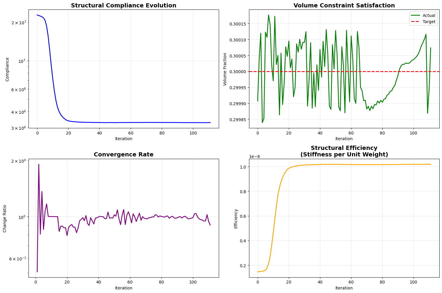
    def plot_performance_metrics(self, history):
        """
        Plot detailed performance metrics.
        """
        fig, ((ax1, ax2), (ax3, ax4)) = plt.subplots(2, 2, figsize=(15, 10))
        
        iterations = range(len(history['compliance']))
        
        # Compliance improvement
        ax1.plot(iterations, history['compliance'], 'b-', linewidth=2)
        ax1.set_title('Structural Compliance Evolution', fontsize=14, fontweight='bold')
        ax1.set_xlabel('Iteration')
        ax1.set_ylabel('Compliance')
        ax1.grid(True, alpha=0.3)
        ax1.set_yscale('log')
        
        # Volume constraint satisfaction
        ax2.plot(iterations, history['volume'], 'g-', linewidth=2, label='Actual')
        ax2.axhline(y=self.volfrac, color='r', linestyle='--', linewidth=2, label='Target')
        ax2.set_title('Volume Constraint Satisfaction', fontsize=14, fontweight='bold')
        ax2.set_xlabel('Iteration')
        ax2.set_ylabel('Volume Fraction')
        ax2.grid(True, alpha=0.3)
        ax2.legend()
        
        # Convergence rate
        if len(history['change']) > 1:
            convergence_rate = np.array(history['change'][1:]) / np.array(history['change'][:-1])
            ax3.semilogy(range(1, len(convergence_rate)+1), convergence_rate, 'purple', linewidth=2)
            ax3.set_title('Convergence Rate', fontsize=14, fontweight='bold')
            ax3.set_xlabel('Iteration')
            ax3.set_ylabel('Change Ratio')
            ax3.grid(True, alpha=0.3)
        
        # Efficiency metric (stiffness per unit weight)
        efficiency = 1.0 / (np.array(history['compliance']) * np.array(history['volume']))
        ax4.plot(iterations, efficiency, 'orange', linewidth=2)
        ax4.set_title('Structural Efficiency\n(Stiffness per Unit Weight)', fontsize=14, fontweight='bold')
        ax4.set_xlabel('Iteration')
        ax4.set_ylabel('Efficiency')
        ax4.grid(True, alpha=0.3)
        
        plt.tight_layout()
        plt.show()

# Run the optimization
print("=" * 60)
print("BONE STRUCTURE OPTIMIZATION SIMULATION")
print("=" * 60)

# Create optimizer instance
optimizer = BoneStructureOptimizer(nelx=80, nely=50, volfrac=0.3, penal=3, rmin=2.0)

# Run optimization
optimal_structure, history, displacements = optimizer.optimize(max_iterations=150)

print("\n" + "=" * 60)
print("OPTIMIZATION COMPLETE - GENERATING VISUALIZATIONS")
print("=" * 60)

# Visualize results
fig = optimizer.visualize_results(optimal_structure, history, displacements)

# Print final analysis
print("\n" + "=" * 60)
print("FINAL ANALYSIS SUMMARY")
print("=" * 60)
print(f"Material usage: {np.sum(optimal_structure)/(optimizer.nelx*optimizer.nely)*100:.1f}%")
print(f"Weight reduction: {(1-optimizer.volfrac)*100:.1f}% compared to solid structure")
print(f"Final compliance: {history['compliance'][-1]:.3e}")
print(f"Optimization converged in {len(history['compliance'])} iterations")
print("\nThis structure demonstrates how bones achieve maximum strength")
print("with minimum weight through optimized internal architecture!")