import matplotlib.pyplot as plt %matplotlib inline
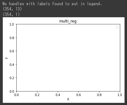
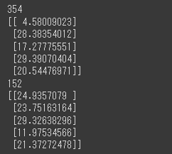
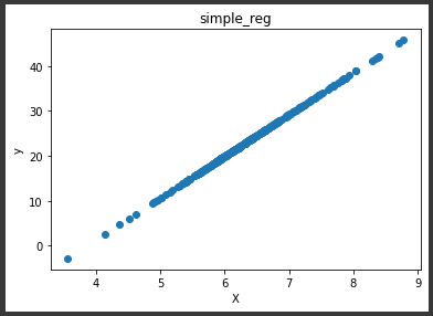
print(X_train.shape) print(y_train_pred.shape) #plt.scatter(X_train, y_train_pred, label="train") # ValueError: x and y must be the same size #plt.scatter(X_test, y_test_pred, label="test") # ValueError: x and y must be the same size plt.xlabel("X") plt.ylabel("y") plt.title("multi_reg") plt.legend() plt.show()
エラーが発生したため、6~7行目をコメントアウトしました。
ValueError: x and y must be the same sizeというエラーメッセージは引数にしている変数の次元数が同じではないために発生したエラーになります。