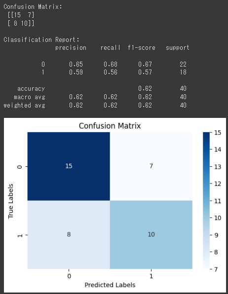
import numpy as np import pandas as pd from sklearn.model_selection import train_test_split from sklearn.ensemble import RandomForestClassifier from sklearn.metrics import confusion_matrix, classification_report import matplotlib.pyplot as plt
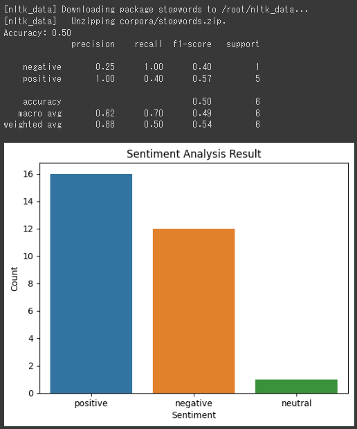
import numpy as np import pandas as pd import matplotlib.pyplot as plt import seaborn as sns import re import nltk from nltk.corpus import stopwords from sklearn.feature_extraction.text import CountVectorizer from sklearn.model_selection import train_test_split from sklearn.naive_bayes import MultinomialNB from sklearn.metrics import accuracy_score, confusion_matrix, classification_report
data = { 'text': [ "I love this product, it's amazing!", "This movie was terrible, never watching it again!", "Neutral tweet about some topic.", "The weather is beautiful today.", "Had a great time at the beach with friends!", "Feeling tired after a long day at work.", "Excited for the upcoming vacation!", "Disappointed with the customer service.", "Trying out a new recipe for dinner tonight.", "Can't wait to see my favorite band in concert!", "Feeling happy and grateful for all the love and support.", "Feeling overwhelmed with deadlines and tasks.", "Just finished reading a fantastic book!", "Feeling bored, looking for something fun to do.", "Feeling anxious about the job interview tomorrow.", "Enjoying a relaxing weekend at home.", "Feeling proud of my accomplishments.", "The traffic today is unbearable!", "Feeling lonely on a rainy day.", "Delighted to meet an old friend unexpectedly.", "Feeling frustrated with the slow internet connection.", "Had a bad experience at the restaurant tonight.", "Feeling motivated to achieve my goals.", "Feeling nostalgic looking at old photos.", "Feeling grateful for the little things in life.", "Feeling sad after saying goodbye to a dear friend.", "Excited for the new season of my favorite TV show!", "Feeling stressed about the upcoming exam.", "The new gadget I bought is not working properly.", ], 'sentiment': [ 'positive', 'negative', 'neutral', 'positive', 'positive', 'negative', 'positive', 'negative', 'positive', 'positive', 'positive', 'negative', 'positive', 'negative', 'negative', 'positive', 'positive', 'negative', 'negative', 'positive', 'negative', 'negative', 'positive', 'positive', 'positive', 'negative', 'positive', 'negative', 'positive' ] }
defpreprocess_text(text): text = re.sub('[^a-zA-Z]', ' ', text) text = text.lower() text = text.split() text = [word for word in text ifnot word in stop_words] text = ' '.join(text) return text
df['text'] = df['text'].apply(preprocess_text)
次に、テキストデータを数値ベクトル化します。
1 2 3
vectorizer = CountVectorizer() X = vectorizer.fit_transform(df['text']) y = df['sentiment']
データセットをトレーニングセットとテストセットに分割します。
1
X_train, X_test, y_train, y_test = train_test_split(X, y, test_size=0.2, random_state=42)
import numpy as np import pandas as pd import matplotlib.pyplot as plt from sklearn.model_selection import train_test_split from sklearn.ensemble import RandomForestClassifier from sklearn.metrics import accuracy_score, confusion_matrix, plot_confusion_matrix
import numpy as np import matplotlib.pyplot as plt from sklearn.datasets import make_multilabel_classification from sklearn.model_selection import train_test_split from sklearn.preprocessing import StandardScaler from sklearn.neighbors import KNeighborsClassifier from sklearn.metrics import accuracy_score, classification_report, confusion_matrix
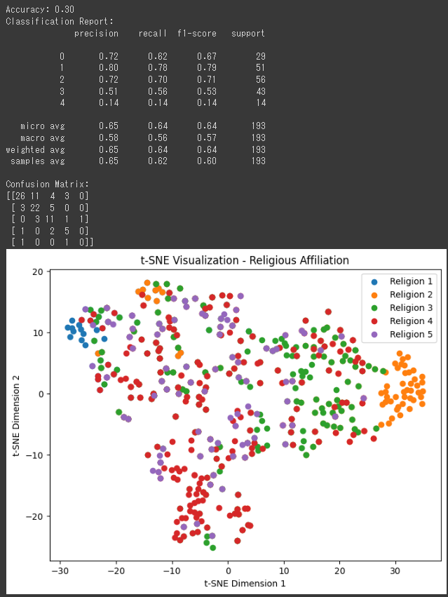
次に、架空の宗教データを作成します。
1 2 3 4 5 6 7 8 9
# 架空の宗教データを生成 X, y = make_multilabel_classification(n_samples=500, n_features=4, n_classes=5, n_labels=2, random_state=42)
# 特徴量のスケーリング scaler = StandardScaler() X = scaler.fit_transform(X)
import pandas as pd import numpy as np import matplotlib.pyplot as plt from sklearn.model_selection import train_test_split from sklearn.ensemble import RandomForestClassifier from sklearn.metrics import accuracy_score, confusion_matrix, roc_curve, roc_auc_score
import numpy as np import matplotlib.pyplot as plt from sklearn.model_selection import train_test_split from sklearn.linear_model import LogisticRegression from sklearn.metrics import accuracy_score, confusion_matrix, classification_report