1
2
3
4
5
6
7
8
9
10
11
12
13
14
15
16
17
18
19
20
21
22
23
24
25
26
27
28
29
30
31
32
33
34
35
36
37
38
39
40
41
42
43
44
45
46
47
48
49
50
51
52
53
54
55
56
57
58
59
60
61
62
63
64
65
66
67
68
69
70
71
72
73
74
75
76
77
78
79
80
81
82
83
84
85
86
87
88
89
90
91
92
93
94
95
96
97
98
99
100
101
102
103
104
105
106
107
108
109
110
111
112
113
114
115
116
117
118
119
120
121
122
123
124
125
126
127
128
129
130
131
132
133
134
135
136
137
138
139
140
141
142
143
144
145
146
147
148
149
150
151
152
153
154
155
156
157
158
159
160
161
162
163
164
165
166
167
168
169
170
171
172
173
174
175
176
177
178
179
180
181
182
183
184
185
186
187
188
189
190
191
192
193
194
195
196
197
198
199
200
201
202
203
204
205
206
207
208
209
210
211
212
213
214
215
216
217
218
219
220
221
222
223
224
225
226
227
228
229
230
231
232
233
234
235
236
237
238
239
240
241
242
243
244
245
246
247
248
249
250
251
252
253
254
255
256
257
258
259
260
261
262
263
264
265
266
267
268
269
270
271
272
273
274
275
276
277
278
279
280
281
282
283
284
285
286
287
288
289
290
| import numpy as np
import matplotlib.pyplot as plt
from matplotlib import cm
from mpl_toolkits.mplot3d import Axes3D
from scipy.integrate import quad
from scipy.optimize import minimize_scalar, minimize
import warnings
warnings.filterwarnings('ignore')
HBAR = 1.0
M = 1.0
OMEGA = 1.0
def E_harmonic_analytical(alpha, hbar=HBAR, m=M, omega=OMEGA):
return (hbar**2 * alpha) / (2 * m) + (m * omega**2) / (8 * alpha)
def trial_psi(x, alpha):
"""Gaussian trial wavefunction (unnormalized core)."""
return np.exp(-alpha * x**2)
def E_numerical(alpha, lam=0.0, hbar=HBAR, m=M, omega=OMEGA, limit=200):
"""
Numerically compute <H> / <psi|psi> for Gaussian trial wavefunction.
Kinetic: <psi| -hbar^2/(2m) d^2/dx^2 |psi>
= hbar^2*alpha/(2m) * sqrt(pi/(2*alpha)) [known analytically]
Potential (harmonic): 0.5*m*omega^2 * <x^2>
= m*omega^2/(8*alpha) * sqrt(pi/alpha) ... combined below
Quartic: lambda * <x^4> -- computed numerically
"""
norm2, _ = quad(lambda x: np.exp(-2*alpha*x**2), -np.inf, np.inf, limit=limit)
T = (hbar**2 / (2*m)) * alpha * norm2
V_harm, _ = quad(lambda x: 0.5*m*omega**2 * x**2 * np.exp(-2*alpha*x**2),
-np.inf, np.inf, limit=limit)
V_quar, _ = quad(lambda x: lam * x**4 * np.exp(-2*alpha*x**2),
-np.inf, np.inf, limit=limit)
return (T + V_harm + V_quar) / norm2
alpha_values = np.linspace(0.1, 3.0, 500)
E_harm = E_harmonic_analytical(alpha_values)
res_harm = minimize_scalar(E_harmonic_analytical, bounds=(0.01, 10), method='bounded')
alpha_opt_harm = res_harm.x
E_opt_harm = res_harm.fun
E_exact_harm = 0.5 * HBAR * OMEGA
LAMBDA = 0.1
E_anharm = np.array([E_numerical(a, lam=LAMBDA) for a in alpha_values])
res_anharm = minimize_scalar(lambda a: E_numerical(a, lam=LAMBDA),
bounds=(0.1, 5.0), method='bounded')
alpha_opt_anharm = res_anharm.x
E_opt_anharm = res_anharm.fun
def exact_ground_state(lam=0.1, N=1000, xmax=10.0):
"""Finite-difference Hamiltonian diagonalization for exact E0."""
x = np.linspace(-xmax, xmax, N)
dx = x[1] - x[0]
diag = (HBAR**2 / (M * dx**2) +
0.5 * M * OMEGA**2 * x**2 + lam * x**4)
off = -HBAR**2 / (2 * M * dx**2) * np.ones(N-1)
H = np.diag(diag) + np.diag(off, 1) + np.diag(off, -1)
eigvals = np.linalg.eigvalsh(H)
return eigvals[0], x, H
E_exact_anharm, x_grid, H_mat = exact_ground_state(LAMBDA)
print(f"=== Harmonic Oscillator ===")
print(f" Optimal alpha : {alpha_opt_harm:.6f} (exact: {M*OMEGA/(2*HBAR):.6f})")
print(f" Variational E0 : {E_opt_harm:.6f}")
print(f" Exact E0 : {E_exact_harm:.6f}")
print(f" Error : {abs(E_opt_harm - E_exact_harm):.2e}")
print()
print(f"=== Anharmonic Oscillator (lambda={LAMBDA}) ===")
print(f" Optimal alpha : {alpha_opt_anharm:.6f}")
print(f" Variational E0 : {E_opt_anharm:.6f}")
print(f" Exact E0 (FD) : {E_exact_anharm:.6f}")
print(f" Error : {abs(E_opt_anharm - E_exact_anharm):.6f}")
print(f" Relative Error (%) : {abs(E_opt_anharm - E_exact_anharm)/E_exact_anharm*100:.4f}%")
def E_2param_numerical(alpha, beta, lam=LAMBDA, limit=100):
"""<H> for 2-parameter trial wavefunction exp(-alpha*x^2 - beta*x^4)."""
if alpha <= 0 or beta <= 0:
return 1e10
def psi2(x):
return np.exp(-2*(alpha*x**2 + beta*x**4))
norm2, _ = quad(psi2, -np.inf, np.inf, limit=limit)
def T_integrand(x):
deriv = (2*alpha + 12*beta*x**2 - (2*alpha*x + 4*beta*x**3)**2)
return 0.5 * deriv * psi2(x)
def V_integrand(x):
return (0.5*OMEGA**2*x**2 + lam*x**4) * psi2(x)
T_val, _ = quad(T_integrand, -np.inf, np.inf, limit=limit)
V_val, _ = quad(V_integrand, -np.inf, np.inf, limit=limit)
return (T_val + V_val) / norm2
a_grid = np.linspace(0.2, 2.0, 40)
b_grid = np.linspace(0.01, 0.5, 40)
AA, BB = np.meshgrid(a_grid, b_grid)
EE = np.zeros_like(AA)
for i in range(AA.shape[0]):
for j in range(AA.shape[1]):
EE[i, j] = E_2param_numerical(AA[i,j], BB[i,j])
res_2p = minimize(lambda p: E_2param_numerical(p[0], p[1]),
x0=[0.5, 0.1], method='Nelder-Mead',
options={'xatol':1e-6,'fatol':1e-6,'maxiter':5000})
alpha2_opt, beta2_opt = res_2p.x
E2_opt = res_2p.fun
print(f"\n=== 2-Parameter Variational (lambda={LAMBDA}) ===")
print(f" Optimal alpha : {alpha2_opt:.6f}")
print(f" Optimal beta : {beta2_opt:.6f}")
print(f" Variational E0 : {E2_opt:.6f}")
print(f" Exact E0 (FD) : {E_exact_anharm:.6f}")
print(f" Relative Error (%) : {abs(E2_opt - E_exact_anharm)/E_exact_anharm*100:.4f}%")
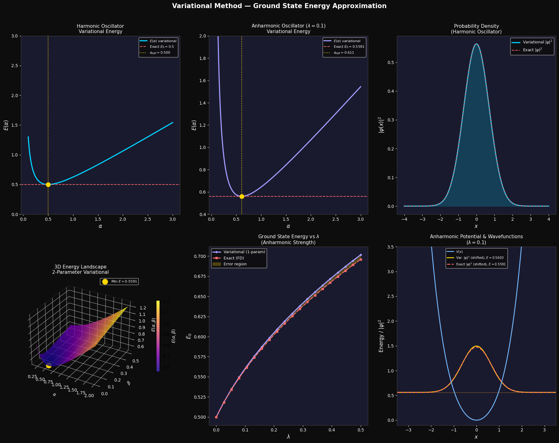
fig = plt.figure(figsize=(18, 14))
fig.patch.set_facecolor('#0d0d0d')
ax1 = fig.add_subplot(2, 3, 1)
ax1.set_facecolor('#1a1a2e')
ax1.plot(alpha_values, E_harm, color='#00d4ff', lw=2.5, label=r'$E(\alpha)$ variational')
ax1.axhline(E_exact_harm, color='#ff6b6b', lw=1.5, ls='--', label=f'Exact $E_0={E_exact_harm}$')
ax1.axvline(alpha_opt_harm, color='#ffd700', lw=1.5, ls=':', label=f'$\\alpha_{{opt}}={alpha_opt_harm:.3f}$')
ax1.scatter([alpha_opt_harm], [E_opt_harm], color='#ffd700', s=100, zorder=5)
ax1.set_xlabel(r'$\alpha$', color='white', fontsize=12)
ax1.set_ylabel(r'$E(\alpha)$', color='white', fontsize=12)
ax1.set_title('Harmonic Oscillator\nVariational Energy', color='white', fontsize=11)
ax1.legend(fontsize=8, facecolor='#0d0d0d', labelcolor='white')
ax1.tick_params(colors='white'); ax1.spines[:].set_color('#444')
ax1.set_ylim(0, 3)
ax2 = fig.add_subplot(2, 3, 2)
ax2.set_facecolor('#1a1a2e')
ax2.plot(alpha_values, E_anharm, color='#a29bfe', lw=2.5, label=r'$E(\alpha)$ variational')
ax2.axhline(E_exact_anharm, color='#ff6b6b', lw=1.5, ls='--',
label=f'Exact $E_0={E_exact_anharm:.4f}$')
ax2.axvline(alpha_opt_anharm, color='#ffd700', lw=1.5, ls=':',
label=f'$\\alpha_{{opt}}={alpha_opt_anharm:.3f}$')
ax2.scatter([alpha_opt_anharm], [E_opt_anharm], color='#ffd700', s=100, zorder=5)
ax2.set_xlabel(r'$\alpha$', color='white', fontsize=12)
ax2.set_ylabel(r'$E(\alpha)$', color='white', fontsize=12)
ax2.set_title(f'Anharmonic Oscillator ($\\lambda={LAMBDA}$)\nVariational Energy', color='white', fontsize=11)
ax2.legend(fontsize=8, facecolor='#0d0d0d', labelcolor='white')
ax2.tick_params(colors='white'); ax2.spines[:].set_color('#444')
ax2.set_ylim(0.4, 2.0)
ax3 = fig.add_subplot(2, 3, 3)
ax3.set_facecolor('#1a1a2e')
x_plot = np.linspace(-4, 4, 500)
norm_harm = (2*alpha_opt_harm/np.pi)**0.25
psi_var = norm_harm * np.exp(-alpha_opt_harm * x_plot**2)
alpha_exact = M*OMEGA/(2*HBAR)
norm_exact = (2*alpha_exact/np.pi)**0.25
psi_exact = norm_exact * np.exp(-alpha_exact * x_plot**2)
ax3.plot(x_plot, psi_var**2, color='#00d4ff', lw=2.5, label='Variational $|\\psi|^2$')
ax3.plot(x_plot, psi_exact**2, color='#ff6b6b', lw=1.5, ls='--', label='Exact $|\\psi|^2$')
ax3.fill_between(x_plot, psi_var**2, alpha=0.2, color='#00d4ff')
ax3.set_xlabel('$x$', color='white', fontsize=12)
ax3.set_ylabel(r'$|\psi(x)|^2$', color='white', fontsize=12)
ax3.set_title('Probability Density\n(Harmonic Oscillator)', color='white', fontsize=11)
ax3.legend(fontsize=9, facecolor='#0d0d0d', labelcolor='white')
ax3.tick_params(colors='white'); ax3.spines[:].set_color('#444')
ax4 = fig.add_subplot(2, 3, 4, projection='3d')
ax4.set_facecolor('#0d0d0d')
EE_clip = np.clip(EE, 0.5, 3.0)
surf = ax4.plot_surface(AA, BB, EE_clip, cmap='plasma', alpha=0.85,
linewidth=0, antialiased=True)
ax4.scatter([alpha2_opt], [beta2_opt], [E2_opt], color='#ffd700',
s=150, zorder=10, label=f'Min $E={E2_opt:.4f}$')
ax4.set_xlabel(r'$\alpha$', color='white', fontsize=10, labelpad=8)
ax4.set_ylabel(r'$\beta$', color='white', fontsize=10, labelpad=8)
ax4.set_zlabel(r'$E(\alpha,\beta)$', color='white', fontsize=10, labelpad=8)
ax4.set_title('3D Energy Landscape\n2-Parameter Variational', color='white', fontsize=11)
ax4.tick_params(colors='white')
ax4.xaxis.pane.fill = False; ax4.yaxis.pane.fill = False; ax4.zaxis.pane.fill = False
ax4.xaxis.pane.set_edgecolor('#333'); ax4.yaxis.pane.set_edgecolor('#333')
ax4.zaxis.pane.set_edgecolor('#333')
ax4.legend(fontsize=8, facecolor='#0d0d0d', labelcolor='white', loc='upper right')
fig.colorbar(surf, ax=ax4, shrink=0.4, pad=0.1,
label='$E(\\alpha,\\beta)$').ax.yaxis.label.set_color('white')
ax5 = fig.add_subplot(2, 3, 5)
ax5.set_facecolor('#1a1a2e')
lambda_arr = np.linspace(0, 0.5, 20)
E_var_lam, E_exa_lam = [], []
for lv in lambda_arr:
rv = minimize_scalar(lambda a: E_numerical(a, lam=lv),
bounds=(0.1, 8.0), method='bounded')
E_var_lam.append(rv.fun)
E_exa_lam.append(exact_ground_state(lv, N=600)[0])
ax5.plot(lambda_arr, E_var_lam, color='#a29bfe', lw=2.5, marker='o',
ms=4, label='Variational (1-param)')
ax5.plot(lambda_arr, E_exa_lam, color='#ff6b6b', lw=2.0, ls='--',
marker='s', ms=4, label='Exact (FD)')
ax5.fill_between(lambda_arr, E_var_lam, E_exa_lam, alpha=0.25, color='#ffd700',
label='Error region')
ax5.set_xlabel(r'$\lambda$', color='white', fontsize=12)
ax5.set_ylabel(r'$E_0$', color='white', fontsize=12)
ax5.set_title('Ground State Energy vs $\\lambda$\n(Anharmonic Strength)', color='white', fontsize=11)
ax5.legend(fontsize=9, facecolor='#0d0d0d', labelcolor='white')
ax5.tick_params(colors='white'); ax5.spines[:].set_color('#444')
ax6 = fig.add_subplot(2, 3, 6)
ax6.set_facecolor('#1a1a2e')
x_p = np.linspace(-3.5, 3.5, 500)
V_anharm_plot = 0.5*OMEGA**2*x_p**2 + LAMBDA*x_p**4
eigvals_full, eigvecs_full = np.linalg.eigh(H_mat)
psi_fd = eigvecs_full[:, 0]
psi_fd /= np.sqrt(np.trapz(psi_fd**2, x_grid))
scale = 0.3 / np.max(np.abs(psi_fd))
psi_var1 = np.exp(-alpha_opt_anharm * x_p**2)
psi_var1 /= np.sqrt(np.trapz(psi_var1**2, x_p))
ax6.plot(x_p, V_anharm_plot, color='#74b9ff', lw=2.0, label='$V(x)$', zorder=3)
ax6.axhline(E_exact_anharm, color='#ff6b6b', lw=1.0, ls=':', alpha=0.7)
ax6.axhline(E_opt_anharm, color='#ffd700', lw=1.0, ls=':', alpha=0.7)
ax6.plot(x_p, psi_var1**2 * 1.5 + E_opt_anharm, color='#ffd700', lw=2.0,
label=f'Var. $|\\psi|^2$ (shifted), $E={E_opt_anharm:.4f}$')
ax6.plot(x_grid, psi_fd**2 * 1.5 + E_exact_anharm, color='#ff6b6b', lw=2.0, ls='--',
label=f'Exact $|\\psi|^2$ (shifted), $E={E_exact_anharm:.4f}$')
ax6.set_xlim(-3.5, 3.5); ax6.set_ylim(-0.1, 3.5)
ax6.set_xlabel('$x$', color='white', fontsize=12)
ax6.set_ylabel('Energy / $|\\psi|^2$', color='white', fontsize=12)
ax6.set_title(f'Anharmonic Potential & Wavefunctions\n($\\lambda={LAMBDA}$)', color='white', fontsize=11)
ax6.legend(fontsize=7.5, facecolor='#0d0d0d', labelcolor='white')
ax6.tick_params(colors='white'); ax6.spines[:].set_color('#444')
plt.suptitle('Variational Method — Ground State Energy Approximation',
color='white', fontsize=15, fontweight='bold', y=1.01)
plt.tight_layout()
plt.savefig('variational_method.png', dpi=150, bbox_inches='tight',
facecolor='#0d0d0d')
plt.show()
print("Figure saved.")
|