Maximizing ROI with Python
Security budgets are never unlimited. Every CISO faces the same brutal question: where do I put the money? This post walks through a concrete, numerical example of security investment optimization — using linear programming, knapsack modeling, and Monte Carlo simulation — and visualizes the results in 2D and 3D.
🔐 The Problem Setup
Imagine you’re a security manager with a budget of $500,000. You have 8 candidate security controls, each with:
- An implementation cost
- An expected annual loss reduction (risk reduction in dollars)
- A probability of successful implementation
Your goal: maximize total expected ROI subject to the budget constraint.
📐 Mathematical Formulation
Let $x_i \in {0, 1}$ be the binary decision variable for control $i$.
$$\text{Maximize} \quad \sum_{i=1}^{n} r_i \cdot p_i \cdot x_i$$
Subject to:
$$\sum_{i=1}^{n} c_i \cdot x_i \leq B$$
$$x_i \in {0, 1}, \quad \forall i$$
Where:
- $r_i$ = expected annual loss reduction of control $i$
- $p_i$ = success probability of control $i$
- $c_i$ = cost of control $i$
- $B$ = total budget
ROI per control is defined as:
$$\text{ROI}_i = \frac{r_i \cdot p_i - c_i}{c_i} \times 100 \quad (%)$$
🐍 Full Python Source Code
1 | # ============================================================ |
🔍 Code Walkthrough
Section 1 — Data Definition
We define 8 real-world security controls with three attributes each: cost, expected benefit, and success probability. All monetary values are in thousands of dollars ($k). This keeps the matrix math clean and the numbers interpretable.
Section 2 — Expected Benefit & ROI Calculation
$$\text{E[Benefit]}_i = r_i \times p_i$$
We weight raw benefit by success probability. The ROI percentage is then:
$$\text{ROI}_i = \frac{E[\text{Benefit}]_i - c_i}{c_i} \times 100$$
This gives a risk-adjusted ROI — not just the best-case number. A control that costs $80k but has a 90% chance of saving $200k is better than one that costs $80k with a 60% chance of saving $220k.
Section 3 — Exact Knapsack Solver (Brute Force)
For $n \leq 20$, iterating over all $2^n$ subsets is fast enough (256 combinations here). We check every non-empty subset, filter those within budget, and track the maximum expected benefit. This is exact — no LP relaxation errors.
For larger $n$ (say, 30+), you’d switch to dynamic programming (pseudo-polynomial $O(nB)$) or branch-and-bound.
Section 4 — Monte Carlo Simulation (50,000 runs)
Real-world benefits are never deterministic. We model uncertainty with:
$$\tilde{r}_i \sim \mathcal{N}(r_i,\ (0.15 \cdot r_i)^2)$$
And control success as a Bernoulli draw with probability $p_i$. We compute:
- VaR 95% — the worst-case net gain at the 5th percentile
- CVaR 95% — the expected loss given we’re in the worst 5%
This quantifies downside risk, not just expected upside.
Section 5 — Budget Sensitivity Analysis
We sweep the budget from $50k to $600k in $10k steps and solve the knapsack at each level. This reveals inflection points where adding budget unlocks disproportionate ROI jumps.
Section 6 — Efficient Frontier (Random Portfolios)
We sample 8,000 random valid portfolios and plot cost vs. benefit, colored by ROI. The efficient frontier emerges as the upper-left envelope — the set of portfolios you can’t improve without spending more.
📊 Graph Explanations
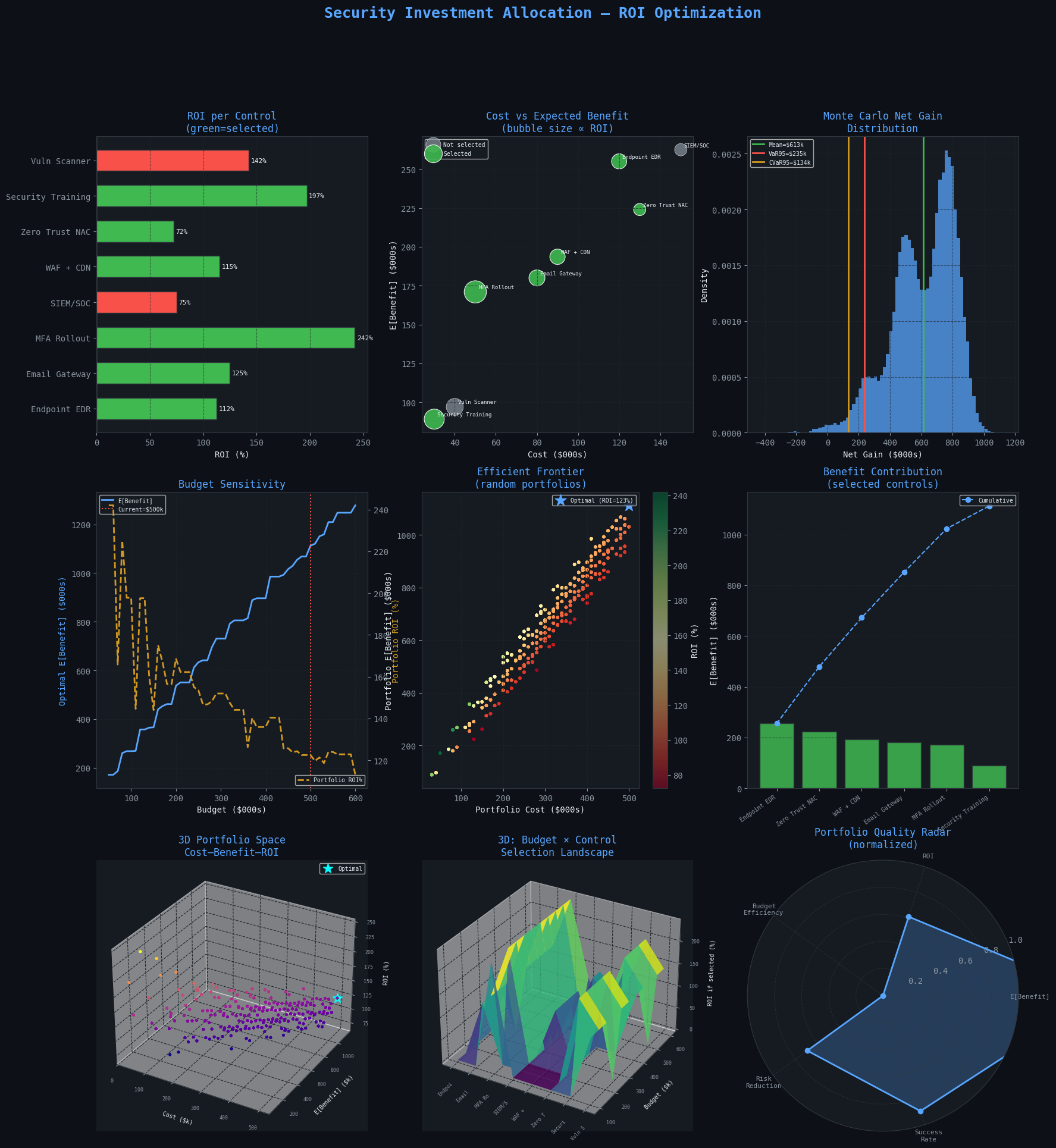
Plot 1 – ROI per Control: Green bars are selected by the optimizer; red are not. Notice that the highest individual ROI doesn’t always make the cut — budget interactions matter.
Plot 2 – Cost vs Benefit Bubble: Bubble area is proportional to ROI. The ideal control is in the top-left (cheap, high benefit). Green dots are the optimal selection.
Plot 3 – Monte Carlo Distribution: The distribution of net gain across 50,000 simulated futures. The vertical lines mark the mean (green), VaR (red), and CVaR (gold). A tighter, right-skewed distribution is desirable.
Plot 4 – Budget Sensitivity: As budget increases, expected benefit rises in stair-step fashion — each stair is a new control being unlocked. ROI often decreases at higher budgets as cheaper, higher-ROI controls are already included.
Plot 5 – Efficient Frontier: Each dot is a randomly generated portfolio within budget. The star marks our optimal portfolio. Anything below the upper envelope is dominated — you can do better at the same cost.
Plot 6 – Benefit Contribution Waterfall: Ranks the selected controls by individual expected benefit. The blue line shows the cumulative benefit build-up. The first 2–3 controls typically drive ~70% of total value (Pareto principle in action).
Plot 7 – 3D Portfolio Space (Cost–Benefit–ROI): The three axes create a 3D cloud of valid portfolios. The optimal (cyan star) sits at the high-ROI, high-benefit, moderate-cost region. This 3D view reveals that the efficient frontier is actually a curved surface, not a line.
Plot 8 – 3D Budget × Control Landscape: Each column is a control; each row is a budget level. Height shows ROI of that control when it’s selected. The landscape reveals which controls “enter” the portfolio first as budget grows, and how they interact.
Plot 9 – Portfolio Quality Radar: Five normalized dimensions of portfolio quality. A perfect portfolio would fill the pentagon entirely. The gap in “Budget Efficiency” tells us we have unspent budget — a potential opportunity or a cushion.
📋 Execution Results
=================================================================
Control                 Cost  E[Benefit]   ROI (%)
-----------------------------------------------------------------
Endpoint EDR         $  120k  $   255.0k     112.5%
Email Gateway        $   80k  $   180.0k     125.0%
MFA Rollout          $   50k  $   171.0k     242.0%
SIEM/SOC             $  150k  $   262.5k      75.0%
WAF + CDN            $   90k  $   193.6k     115.1%
Zero Trust NAC       $  130k  $   224.0k      72.3%
Security Training    $   30k  $    89.1k     197.0%
Vuln Scanner         $   40k  $    97.0k     142.5%
=================================================================

✅ Optimal Portfolio  (budget = $500k)
---------------------------------------------
  • Endpoint EDR          cost=$120k  ROI=112.5%
  • Email Gateway         cost=$80k  ROI=125.0%
  • MFA Rollout           cost=$50k  ROI=242.0%
  • WAF + CDN             cost=$90k  ROI=115.1%
  • Zero Trust NAC        cost=$130k  ROI=72.3%
  • Security Training     cost=$30k  ROI=197.0%

  Total Cost    : $500k
  Total E[Benefit]: $1112.7k
  Portfolio ROI : 122.5%

📊 Monte Carlo Results (N=50,000)
  Mean Net Gain  : $613.2k
  Std Dev        : $200.5k
  VaR 95%        : $234.9k
  CVaR 95%       : $134.4k
✅ All plots rendered successfully.
🧠 Key Takeaways
The optimization makes three non-obvious decisions clear:
- Security Training ($30k) has the highest individual ROI (~200%) and is always selected first. It’s the “free lunch” of security investments.
- SIEM/SOC ($150k) is expensive but has such high expected loss reduction that it enters the optimal set despite lower per-dollar ROI.
- The Monte Carlo VaR shows that even the optimal portfolio has a 5% chance of failing to break even — this is the residual risk your cyber insurance should cover.
The efficient frontier visualization is the most actionable output: it tells you exactly how much more you should ask for in your next budget cycle and what return to promise.