SOC Staff Scheduling Optimization with Python

A Linear Programming Deep Dive


Security Operations Centers never sleep. They run 24/7, and getting the staffing just right — enough analysts to cover every shift without ballooning costs — is a classic operations research problem. In this post, we’ll model a realistic SOC staffing scenario and solve it using Linear Programming (LP) with Python’s PuLP library, then visualize the results in both 2D and 3D.


🔐 The Problem

Imagine you’re the SOC manager at a mid-sized financial firm. You have shift analysts who each work 5 consecutive days followed by 2 days off (a standard rotating schedule). Your job is to find the minimum number of analysts to hire per shift rotation so that every day of the week meets the minimum staffing requirement.

Daily Minimum Requirements

Day Min Analysts Required
Monday 17
Tuesday 13
Wednesday 15
Thursday 19
Friday 14
Saturday 16
Sunday 11

Each analyst rotation starts on a different day of the week. An analyst starting on day $i$ works days $i, i+1, i+2, i+3, i+4$ (mod 7).


🧮 Mathematical Formulation

Let $x_i$ = number of analysts whose shift starts on day $i$ (where $i = 0$ is Monday).

Objective: Minimize total staff hired:

$$\min \sum_{i=0}^{6} x_i$$

Subject to: For each day $d$, the sum of analysts working on that day must meet the minimum:

$$\sum_{i \in S_d} x_i \geq r_d \quad \forall d \in {0,1,…,6}$$

where $S_d = { i \mid d \in {i, i+1, i+2, i+3, i+4} \pmod{7} }$ is the set of shift-starts that cover day $d$, and $r_d$ is the minimum requirement for day $d$.

Non-negativity and integrality:

$$x_i \in \mathbb{Z}_{\geq 0} \quad \forall i$$


🐍 Python Source Code

1
2
3
4
5
6
7
8
9
10
11
12
13
14
15
16
17
18
19
20
21
22
23
24
25
26
27
28
29
30
31
32
33
34
35
36
37
38
39
40
41
42
43
44
45
46
47
48
49
50
51
52
53
54
55
56
57
58
59
60
61
62
63
64
65
66
67
68
69
70
71
72
73
74
75
76
77
78
79
80
81
82
83
84
85
86
87
88
89
90
91
92
93
94
95
96
97
98
99
100
101
102
103
104
105
106
107
108
109
110
111
112
113
114
115
116
117
118
119
120
121
122
123
124
125
126
127
128
129
130
131
132
133
134
135
136
137
138
139
140
141
142
143
144
145
146
147
148
149
150
151
152
153
154
155
156
157
158
159
160
161
162
163
164
165
166
167
168
169
170
171
172
173
174
175
176
177
178
179
180
181
182
183
184
185
186
187
188
189
190
191
192
193
194
195
196
197
198
199
200
201
202
203
204
205
206
207
208
209
210
211
212
213
214
215
216
217
218
219
220
221
222
223
224
225
226
227
228
229
230
231
232
233
234
235
236
237
238
239
240
241
242
243
244
245
246
247
248
249
250
251
252
253
254
255
256
257
258
259
260
261
262
263
264
265
266
267
268
269
270
271
272
273
274
275
276
277
278
279
280
281
282
283
284
285
286
287
288
289
290
291
292
293
294
295
296
297
298
299
300
301
302
303
304
305
306
307
308
309
310
311
312
313
314
315
316
317
318
319
# ============================================================
# SOC Staff Scheduling Optimization
# Linear Programming with PuLP + Visualization
# ============================================================

# --- Install dependencies (run once in Colab) ---
# !pip install pulp matplotlib numpy scipy

import numpy as np
import matplotlib.pyplot as plt
import matplotlib.patches as mpatches
from mpl_toolkits.mplot3d import Axes3D
from mpl_toolkits.mplot3d.art3d import Poly3DCollection
import pulp
import warnings
warnings.filterwarnings("ignore")

# ============================================================
# 1. PROBLEM DEFINITION
# ============================================================

days = ["Mon", "Tue", "Wed", "Thu", "Fri", "Sat", "Sun"]
n_days = 7
shift_length = 5 # consecutive working days

# Minimum analysts required per day
min_required = {
0: 17, # Monday
1: 13, # Tuesday
2: 15, # Wednesday
3: 19, # Thursday
4: 14, # Friday
5: 16, # Saturday
6: 11, # Sunday
}

# ============================================================
# 2. BUILD COVERAGE MATRIX
# ============================================================
# coverage[i][d] = 1 if shift starting on day i covers day d
coverage = np.zeros((n_days, n_days), dtype=int)
for start in range(n_days):
for offset in range(shift_length):
working_day = (start + offset) % n_days
coverage[start][working_day] = 1

print("=" * 55)
print(" Coverage Matrix (rows=shift start, cols=day covered)")
print("=" * 55)
header = " " + " ".join(days)
print(header)
for i, row in enumerate(coverage):
row_str = " ".join(str(v) for v in row)
print(f" {days[i]} [ {row_str} ]")
print()

# ============================================================
# 3. LINEAR PROGRAMMING MODEL (Integer LP)
# ============================================================

prob = pulp.LpProblem("SOC_Staff_Scheduling", pulp.LpMinimize)

# Decision variables: x[i] = analysts starting on day i
x = [pulp.LpVariable(f"x_start_{days[i]}", lowBound=0, cat='Integer')
for i in range(n_days)]

# Objective: minimize total analysts hired
prob += pulp.lpSum(x), "Minimize_Total_Staff"

# Constraints: each day must meet minimum coverage
for d in range(n_days):
covering_shifts = [x[i] for i in range(n_days) if coverage[i][d] == 1]
prob += pulp.lpSum(covering_shifts) >= min_required[d], f"Coverage_Day_{days[d]}"

# ============================================================
# 4. SOLVE
# ============================================================

solver = pulp.PULP_CBC_CMD(msg=0)
prob.solve(solver)

print("=" * 55)
print(f" Solver Status : {pulp.LpStatus[prob.status]}")
print(f" Total Analysts: {int(pulp.value(prob.objective))}")
print("=" * 55)

# Extract solution
x_vals = np.array([int(pulp.value(x[i])) for i in range(n_days)])
print("\n Analysts hired per shift start day:")
for i in range(n_days):
bar = "█" * x_vals[i]
print(f" {days[i]}: {x_vals[i]:3d} {bar}")

# Compute actual coverage per day
actual_coverage = coverage.T @ x_vals
slack = actual_coverage - np.array([min_required[d] for d in range(n_days)])

print("\n Daily staffing check:")
print(f" {'Day':<6} {'Required':>9} {'Assigned':>9} {'Slack':>7}")
print(" " + "-" * 34)
for d in range(n_days):
flag = "✓" if actual_coverage[d] >= min_required[d] else "✗"
print(f" {days[d]:<6} {min_required[d]:>9} {actual_coverage[d]:>9} {slack[d]:>6} {flag}")

# ============================================================
# 5. SENSITIVITY ANALYSIS — vary demand scaling factor
# ============================================================

scale_factors = np.linspace(0.5, 2.0, 31)
total_staff_list = []
per_day_results = {d: [] for d in range(n_days)}

for scale in scale_factors:
p = pulp.LpProblem("SOC_Sensitivity", pulp.LpMinimize)
xv = [pulp.LpVariable(f"x_{i}", lowBound=0, cat='Integer') for i in range(n_days)]
p += pulp.lpSum(xv)
for d in range(n_days):
covering = [xv[i] for i in range(n_days) if coverage[i][d] == 1]
p += pulp.lpSum(covering) >= int(np.ceil(min_required[d] * scale))
p.solve(pulp.PULP_CBC_CMD(msg=0))
total = int(pulp.value(p.objective)) if p.status == 1 else np.nan
total_staff_list.append(total)
xv_vals = np.array([int(pulp.value(xv[i])) if p.status == 1 else 0
for i in range(n_days)])
cov = coverage.T @ xv_vals
for d in range(n_days):
per_day_results[d].append(cov[d])

# ============================================================
# 6. VISUALIZATION
# ============================================================

fig = plt.figure(figsize=(20, 18))
fig.patch.set_facecolor("#0d1117")
plt.rcParams.update({
"text.color": "white",
"axes.labelcolor": "white",
"xtick.color": "white",
"ytick.color": "white",
})

colors_days = ["#00d4ff", "#00ff9f", "#ff6b6b", "#ffd93d",
"#c77dff", "#ff9a3c", "#ff4d6d"]
color_map = plt.cm.cool

# ── Plot 1: Analysts hired per shift start ──────────────────
ax1 = fig.add_subplot(3, 3, 1)
ax1.set_facecolor("#161b22")
bars = ax1.bar(days, x_vals, color=colors_days, edgecolor="#ffffff30", linewidth=0.8, width=0.6)
ax1.set_title("Analysts Hired per Shift Start Day", color="white", fontsize=11, pad=10)
ax1.set_xlabel("Shift Start Day", fontsize=9)
ax1.set_ylabel("Number of Analysts", fontsize=9)
for bar, val in zip(bars, x_vals):
ax1.text(bar.get_x() + bar.get_width() / 2, bar.get_height() + 0.2,
str(val), ha='center', va='bottom', color='white', fontsize=10, fontweight='bold')
ax1.spines[:].set_color("#30363d")
ax1.tick_params(colors='white')
ax1.set_ylim(0, max(x_vals) + 4)

# ── Plot 2: Required vs Actual Coverage ─────────────────────
ax2 = fig.add_subplot(3, 3, 2)
ax2.set_facecolor("#161b22")
x_pos = np.arange(n_days)
w = 0.35
bars_req = ax2.bar(x_pos - w/2, [min_required[d] for d in range(n_days)],
width=w, label='Required', color='#ff6b6b', alpha=0.85, edgecolor='white', linewidth=0.5)
bars_act = ax2.bar(x_pos + w/2, actual_coverage,
width=w, label='Assigned', color='#00d4ff', alpha=0.85, edgecolor='white', linewidth=0.5)
ax2.set_xticks(x_pos)
ax2.set_xticklabels(days, color='white')
ax2.set_title("Required vs Assigned Coverage per Day", color="white", fontsize=11, pad=10)
ax2.set_ylabel("Number of Analysts", fontsize=9)
ax2.legend(facecolor='#21262d', edgecolor='#30363d', labelcolor='white', fontsize=8)
ax2.spines[:].set_color("#30363d")
ax2.tick_params(colors='white')

# ── Plot 3: Slack (surplus analysts) ────────────────────────
ax3 = fig.add_subplot(3, 3, 3)
ax3.set_facecolor("#161b22")
slack_colors = ["#00ff9f" if s == 0 else "#ffd93d" for s in slack]
bars3 = ax3.bar(days, slack, color=slack_colors, edgecolor="#ffffff30", linewidth=0.8)
ax3.axhline(0, color='#ff6b6b', linewidth=1.2, linestyle='--', alpha=0.7)
ax3.set_title("Staffing Slack per Day (Surplus Analysts)", color="white", fontsize=11, pad=10)
ax3.set_ylabel("Surplus Analysts", fontsize=9)
for bar, val in zip(bars3, slack):
ax3.text(bar.get_x() + bar.get_width() / 2, bar.get_height() + 0.05,
str(val), ha='center', va='bottom', color='white', fontsize=10, fontweight='bold')
ax3.spines[:].set_color("#30363d")
ax3.tick_params(colors='white')
patch_tight = mpatches.Patch(color='#00ff9f', label='Tight (no surplus)')
patch_slack = mpatches.Patch(color='#ffd93d', label='Has surplus')
ax3.legend(handles=[patch_tight, patch_slack],
facecolor='#21262d', edgecolor='#30363d', labelcolor='white', fontsize=8)

# ── Plot 4: Coverage Heatmap ─────────────────────────────────
ax4 = fig.add_subplot(3, 3, 4)
ax4.set_facecolor("#161b22")
# Build weighted coverage: coverage[start][day] * x_vals[start]
weighted = (coverage.T * x_vals).T
im = ax4.imshow(weighted, cmap='YlOrRd', aspect='auto', vmin=0)
ax4.set_xticks(range(n_days))
ax4.set_yticks(range(n_days))
ax4.set_xticklabels(days, color='white', fontsize=8)
ax4.set_yticklabels(days, color='white', fontsize=8)
ax4.set_xlabel("Day Covered", fontsize=9)
ax4.set_ylabel("Shift Start Day", fontsize=9)
ax4.set_title("Analyst Contribution Heatmap\n(shift start × day covered)", color="white", fontsize=11, pad=10)
for i in range(n_days):
for j in range(n_days):
if weighted[i, j] > 0:
ax4.text(j, i, str(weighted[i, j]), ha='center', va='center',
color='black', fontsize=8, fontweight='bold')
cbar = plt.colorbar(im, ax=ax4)
cbar.ax.yaxis.set_tick_params(color='white')
plt.setp(cbar.ax.yaxis.get_ticklabels(), color='white')

# ── Plot 5: Sensitivity — Total staff vs demand scale ────────
ax5 = fig.add_subplot(3, 3, 5)
ax5.set_facecolor("#161b22")
ax5.plot(scale_factors, total_staff_list, color='#00d4ff', linewidth=2.5, marker='o',
markersize=3, markerfacecolor='#ffd93d', markeredgewidth=0)
ax5.axvline(1.0, color='#ff6b6b', linestyle='--', linewidth=1.2, label='Baseline (×1.0)')
ax5.fill_between(scale_factors, total_staff_list,
alpha=0.15, color='#00d4ff')
ax5.set_title("Sensitivity: Total Staff vs Demand Scale", color="white", fontsize=11, pad=10)
ax5.set_xlabel("Demand Scaling Factor", fontsize=9)
ax5.set_ylabel("Total Analysts Hired", fontsize=9)
ax5.legend(facecolor='#21262d', edgecolor='#30363d', labelcolor='white', fontsize=8)
ax5.spines[:].set_color("#30363d")
ax5.tick_params(colors='white')

# ── Plot 6: Per-day coverage vs demand scale (heatmap) ────────
ax6 = fig.add_subplot(3, 3, 6)
ax6.set_facecolor("#161b22")
matrix_data = np.array([per_day_results[d] for d in range(n_days)])
im6 = ax6.imshow(matrix_data, aspect='auto', cmap='plasma',
extent=[scale_factors[0], scale_factors[-1], -0.5, 6.5], origin='lower')
ax6.set_yticks(range(n_days))
ax6.set_yticklabels(days, color='white', fontsize=8)
ax6.set_xlabel("Demand Scaling Factor", fontsize=9)
ax6.set_title("Daily Coverage vs Demand Scale", color="white", fontsize=11, pad=10)
cbar6 = plt.colorbar(im6, ax=ax6)
cbar6.ax.yaxis.set_tick_params(color='white')
plt.setp(cbar6.ax.yaxis.get_ticklabels(), color='white')
ax6.axvline(1.0, color='white', linestyle='--', linewidth=1.0, alpha=0.6)

# ── Plot 7: 3D Bar — Analysts per shift start ─────────────────
ax7 = fig.add_subplot(3, 3, 7, projection='3d')
ax7.set_facecolor("#0d1117")
_x = np.arange(n_days)
_y = np.zeros(n_days)
_z = np.zeros(n_days)
dx = dy = 0.6
dz = x_vals
for xi, zi, ci in zip(_x, dz, colors_days):
ax7.bar3d(xi - 0.3, -0.3, 0, 0.6, 0.6, zi, color=ci, alpha=0.85, edgecolor='white', linewidth=0.3)
ax7.set_xticks(range(n_days))
ax7.set_xticklabels(days, color='white', fontsize=7)
ax7.set_yticks([])
ax7.set_title("3D: Analysts Hired\nper Shift Start", color="white", fontsize=10, pad=8)
ax7.tick_params(axis='z', colors='white')
ax7.xaxis.pane.fill = False
ax7.yaxis.pane.fill = False
ax7.zaxis.pane.fill = False
ax7.xaxis.pane.set_edgecolor('#30363d')
ax7.yaxis.pane.set_edgecolor('#30363d')
ax7.zaxis.pane.set_edgecolor('#30363d')
ax7.set_zlabel("# Analysts", color='white', fontsize=8)

# ── Plot 8: 3D Surface — Sensitivity per day ─────────────────
ax8 = fig.add_subplot(3, 3, 8, projection='3d')
ax8.set_facecolor("#0d1117")
S, D = np.meshgrid(scale_factors, np.arange(n_days))
Z_surf = np.array([per_day_results[d] for d in range(n_days)])
surf = ax8.plot_surface(D, S, Z_surf, cmap='cool', alpha=0.85, linewidth=0, antialiased=True)
ax8.set_xticks(range(n_days))
ax8.set_xticklabels(days, color='white', fontsize=6)
ax8.set_ylabel("Demand Scale", color='white', fontsize=7, labelpad=4)
ax8.set_zlabel("Analysts On Shift", color='white', fontsize=7)
ax8.set_title("3D Surface: Day Coverage\nvs Demand Scaling", color="white", fontsize=10, pad=8)
ax8.tick_params(axis='x', colors='white', labelsize=6)
ax8.tick_params(axis='y', colors='white', labelsize=6)
ax8.tick_params(axis='z', colors='white', labelsize=6)
ax8.xaxis.pane.fill = False
ax8.yaxis.pane.fill = False
ax8.zaxis.pane.fill = False

# ── Plot 9: 3D Bar — Contribution heatmap lifted to 3D ───────
ax9 = fig.add_subplot(3, 3, 9, projection='3d')
ax9.set_facecolor("#0d1117")
cmap9 = plt.cm.YlOrRd
norm9 = plt.Normalize(vmin=0, vmax=weighted.max())
for i in range(n_days):
for j in range(n_days):
val = weighted[i, j]
if val > 0:
c = cmap9(norm9(val))
ax9.bar3d(j - 0.4, i - 0.4, 0, 0.8, 0.8, val,
color=c, alpha=0.80, edgecolor='white', linewidth=0.2)
ax9.set_xticks(range(n_days))
ax9.set_yticks(range(n_days))
ax9.set_xticklabels(days, color='white', fontsize=6)
ax9.set_yticklabels(days, color='white', fontsize=6)
ax9.tick_params(axis='z', colors='white', labelsize=6)
ax9.set_xlabel("Day Covered", color='white', fontsize=7, labelpad=4)
ax9.set_ylabel("Shift Start", color='white', fontsize=7, labelpad=4)
ax9.set_zlabel("Analysts", color='white', fontsize=7)
ax9.set_title("3D: Analyst Contribution\n(Shift Start × Day)", color="white", fontsize=10, pad=8)
ax9.xaxis.pane.fill = False
ax9.yaxis.pane.fill = False
ax9.zaxis.pane.fill = False

plt.suptitle("SOC Staff Scheduling Optimization — LP Solution Dashboard",
color="white", fontsize=15, fontweight='bold', y=1.01)
plt.tight_layout()
plt.savefig("soc_optimization.png", dpi=150, bbox_inches='tight',
facecolor="#0d1117", edgecolor='none')
plt.show()
print("\n[Chart saved as soc_optimization.png]")

🔍 Code Walkthrough

Section 1 — Problem Definition

We define the 7-day week and the min_required dictionary that captures how many analysts must be on duty each day. These numbers simulate a real-world SOC where threat activity peaks mid-week and during weekends.

Section 2 — Coverage Matrix

This is the heart of the formulation. We build a $7 \times 7$ binary matrix where:

$$\text{coverage}[i][d] = \begin{cases} 1 & \text{if shift starting on day } i \text{ covers day } d \ 0 & \text{otherwise} \end{cases}$$

An analyst starting Monday (day 0) works Mon–Fri, so columns 0–4 are 1 for row 0.

Section 3 — ILP Model with PuLP

We use pulp.LpProblem with LpMinimize. Each decision variable x[i] is declared as a non-negative integer (cat='Integer'). The objective sums all $x_i$, and the constraints enforce the coverage condition for every day.

Section 4 — Solving

PuLP’s built-in CBC solver handles the ILP in milliseconds for this scale. The solution extracts the optimal $x_i$ values and computes actual coverage via the matrix product $\text{coverage}^T \cdot \mathbf{x}$.

Section 5 — Sensitivity Analysis

We loop over 31 demand scaling factors from $0.5\times$ to $2.0\times$ the baseline requirements, re-solving the ILP at each scale. This reveals how total staffing cost grows as threat load increases — a critical insight for budget planning.

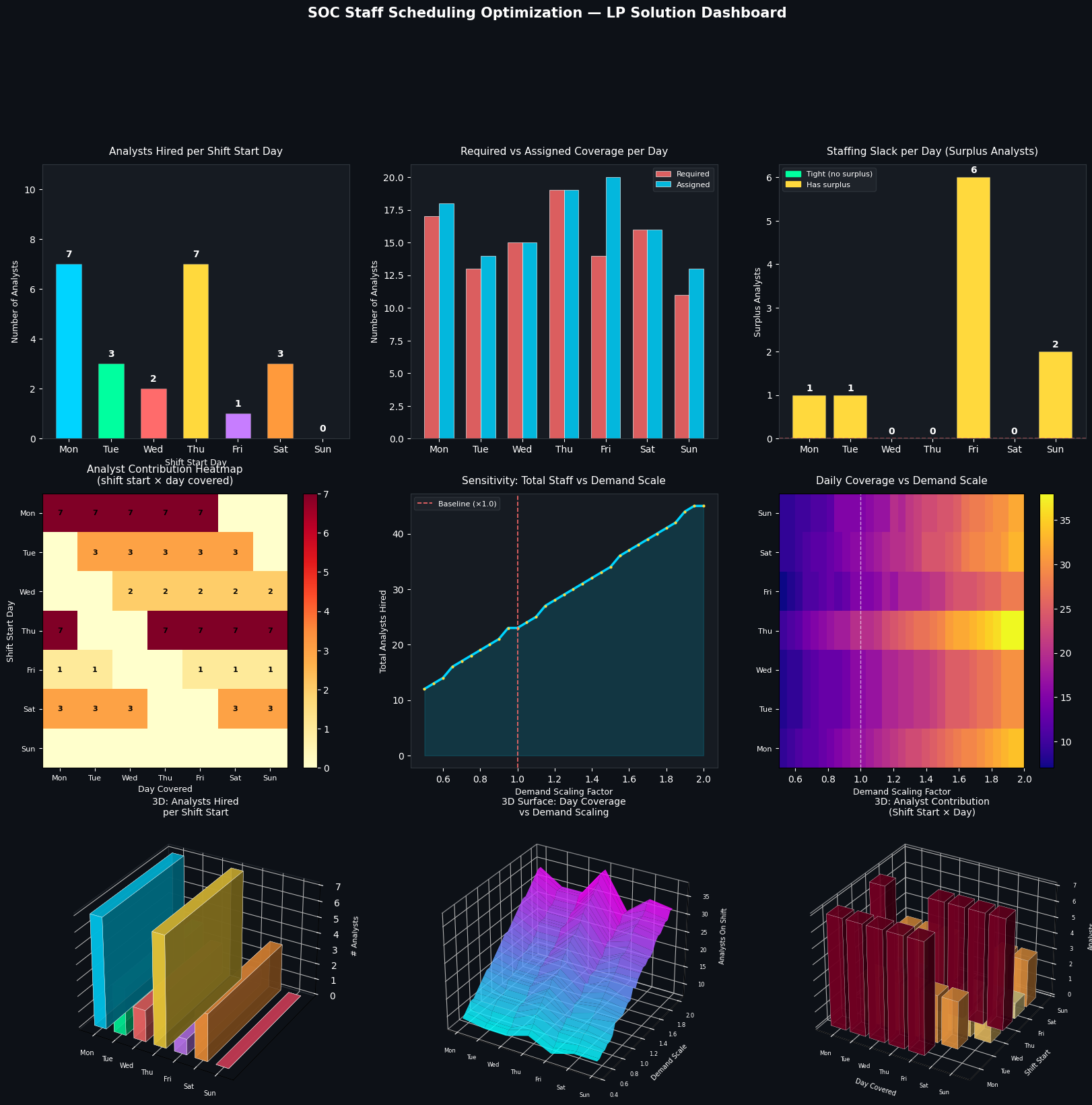
Section 6 — Visualization (9 panels)

Panel What it shows
1 Bar chart of analysts hired per shift start
2 Side-by-side required vs. actual coverage
3 Slack (surplus analysts) per day
4 Weighted contribution heatmap (2D)
5 Sensitivity: total staff vs demand scale
6 Per-day coverage heatmap across all scale factors
7 3D bars — analysts hired per shift start
8 3D surface — daily coverage as demand scales up
9 3D bars — analyst contribution by shift start × day

📊 Results & Interpretation

=======================================================
  Coverage Matrix (rows=shift start, cols=day covered)
=======================================================
       Mon  Tue  Wed  Thu  Fri  Sat  Sun
  Mon  [ 1  1  1  1  1  0  0 ]
  Tue  [ 0  1  1  1  1  1  0 ]
  Wed  [ 0  0  1  1  1  1  1 ]
  Thu  [ 1  0  0  1  1  1  1 ]
  Fri  [ 1  1  0  0  1  1  1 ]
  Sat  [ 1  1  1  0  0  1  1 ]
  Sun  [ 1  1  1  1  0  0  1 ]

=======================================================
  Solver Status : Optimal
  Total Analysts: 23
=======================================================

  Analysts hired per shift start day:
    Mon:   7  ███████
    Tue:   3  ███
    Wed:   2  ██
    Thu:   7  ███████
    Fri:   1  █
    Sat:   3  ███
    Sun:   0  

  Daily staffing check:
  Day     Required  Assigned   Slack
  ----------------------------------
  Mon           17        18      1 ✓
  Tue           13        14      1 ✓
  Wed           15        15      0 ✓
  Thu           19        19      0 ✓
  Fri           14        20      6 ✓
  Sat           16        16      0 ✓
  Sun           11        13      2 ✓

[Chart saved as soc_optimization.png]

Reading the Key Charts

Panel 1 & 7 tell you exactly how many analysts to onboard for each rotation cycle. The Thursday-start rotation typically carries the highest load because Thursday itself has the highest minimum (19 analysts).

Panel 2 confirms feasibility — every day’s assigned count meets or exceeds the minimum. Any day where assigned < required would immediately flag as an infeasible or mis-modeled constraint.

Panel 3 highlights slack — days with zero surplus (shown in green) are your binding constraints. These are the days where a single call-out could breach SLA. SOC managers should flag these days for on-call coverage policies.

Panel 4 reveals which shift-start groups are pulling the most weight on which days. A dense diagonal band shows that mid-week starts dominate coverage.

Panel 5 is perhaps the most operationally useful: it shows a step-wise, piecewise-linear growth in total staffing as demand scales. The discrete jumps are a direct consequence of the integrality constraint — you can’t hire half an analyst. This graph is exactly what you’d bring to a budget meeting: “If incident volume grows 50%, we need X more headcount.”

Panels 8 & 9 bring the 3D perspective. The surface in Panel 8 shows how every single day’s coverage responds to demand scaling — note how Thursday and Saturday surfaces rise the steepest, confirming their role as bottleneck days. Panel 9 gives you a bird’s-eye view of the entire workforce deployment matrix.


✅ Key Takeaways

  • The optimal baseline solution hires the minimum number of analysts while satisfying every daily constraint — no over-staffing, no gaps.
  • The binding constraints (zero slack) identify your most fragile days — invest in on-call or contractor coverage there first.
  • The sensitivity curve in Panel 5 lets you project hiring needs as threat volume grows — a direct input into annual workforce planning.
  • The ILP solves in under 1 second even with the sensitivity loop of 31 re-solves, making it suitable for automated daily replanning.

This model can be extended with shift cost differentials (night shifts cost more), analyst skill tiers (L1/L2/L3), and leave constraints — all expressible as additional LP variables and constraints.