A Practical Python Guide
Log management is one of those things that quietly drains your cloud budget if you’re not paying attention. In this post, we’ll work through a concrete optimization problem — figuring out the ideal log retention period that balances compliance requirements, operational value, and storage cost — and solve it entirely in Python with rich visualizations including 3D plots.
The Problem Setup
Imagine you run a web service generating logs continuously. You need to decide how long to keep logs across multiple storage tiers:
| Tier | Description | Cost (per GB/month) |
|---|---|---|
| Hot | SSD / live storage | $0.023 |
| Warm | HDD / infrequent access | $0.010 |
| Cold | Glacier / archive | $0.004 |
Logs have a decay in operational value over time — a fresh log is invaluable for debugging, but a 2-year-old log is rarely touched. We model this with an exponential decay function.
Total cost over a retention window $T$ (in days):
$$C(T) = \sum_{t=0}^{T} r(t) \cdot p(t) \cdot \Delta t$$
Where:
- $r(t)$ = data volume at time $t$ (GB)
- $p(t)$ = price per GB at tier assigned to time $t$
- $\Delta t$ = time step (1 day)
Operational value decays exponentially:
$$V(t) = V_0 \cdot e^{-\lambda t}$$
Where $\lambda$ is the decay constant. The value-to-cost ratio (efficiency):
$$E(T) = \frac{\int_0^T V(t),dt}{C(T)}$$
We want to find the $T^*$ that maximizes $E(T)$ subject to a minimum compliance window.
Full Python Source Code
1 | # ============================================================ |
Code Walkthrough
Section 1 — Parameters
Everything lives in one place at the top. LAMBDA_DECAY = 0.02 means the log’s operational value halves roughly every 35 days ($t_{1/2} = \ln 2 / \lambda \approx 35$). The three storage tiers mirror real-world AWS S3 pricing (Standard → Infrequent Access → Glacier).
Section 2 — tier_cost_per_gb_day and compute_metrics
tier_cost_per_gb_day(t) uses NumPy boolean masking to vectorize the tier lookup — no Python loop over individual days.
compute_metrics computes three quantities:
- Daily cost:
DAILY_LOG_GB × cost_per_gb_per_day(t) - Daily value: $V_0 \cdot e^{-\lambda t}$ — the exponential decay model
- Cumulative trapezoids:
scipy.integrate.cumulative_trapezoidgives a running numerical integral without any explicit loop, making it fast even at 730-day resolution
The efficiency $E(T) = \text{cum_value}(T) / \text{cum_cost}(T)$ is the metric we optimize.
Section 3 — Sensitivity Analysis (the nested loop)
This is the heaviest block: a 40×40 grid sweep over λ and daily log volume. For each combination, it recomputes the full 640-day arrays and records which day maximizes efficiency (subject to the compliance floor).
Two output matrices are produced:
opt_retention[i,j]— the optimal $T^*$ for parameter pair $(i,j)$opt_efficiency[i,j]— the peak efficiency at that $T^*$
These feed directly into the two 3D surface plots.
Performance note: the inner loop is 1,600 iterations × 640 days = ~1M operations. NumPy vectorization keeps this well under 5 seconds on Colab without needing multiprocessing, but if you push the grid to 100×100, wrap the inner body with
joblib.Parallel.
Section 4 — Finding $T^*$ for the Base Case
After filtering days below the compliance minimum (90 days), idxmax() on the efficiency column finds the optimal retention period. The result is printed immediately so you see the answer before any plotting.
Section 5 — Tier Cost Breakdown
We integrate daily cost separately within each tier’s date range using np.trapz to show how much of the total bill comes from Hot vs. Warm vs. Cold storage. This feeds the pie chart.
Section 6 — Six-Panel Figure
| Panel | What it shows |
|---|---|
| Top-left | Daily cost (red) and daily value decay (green) on dual axes |
| Top-right | Efficiency curve — the key optimization result with $T^*$ marked |
| Mid-left | Cumulative cost and value as filled area charts |
| Mid-right | Pie chart of cost breakdown across tiers at $T^*$ |
| Bottom-left | 3D surface: how $T^*$ changes with decay rate and log volume |
| Bottom-right | 3D surface: how peak efficiency changes with the same parameters |
Graph Explanations
Efficiency curve (top-right) is the heart of the analysis. It rises quickly in the early days because you’re accumulating value faster than cost. Once the log value has decayed significantly, each additional day of retention costs more than it’s worth — so the curve bends down. The red dashed line marks $T^*$, the exact inflection you want to set your retention policy at.
Cumulative cost vs. value (mid-left) makes the crossover intuitive: as long as the green area grows faster than the red area, extending retention is a net positive.
Tier cost pie (mid-right) often surprises teams — despite Cold storage being the cheapest per GB, logs accumulate in that tier for the longest time, and it can still account for a significant slice of total spend.
3D optimal retention surface (bottom-left) is the most policy-relevant chart. It shows that:
- Higher decay rates $\lambda$ → shorter optimal $T^*$ (logs lose value fast, so archive or delete sooner)
- Higher log volume → doesn’t fundamentally shift $T^*$ because cost and value scale proportionally — the ratio stays similar
3D efficiency surface (bottom-right) complements this by showing that teams with rapidly decaying, low-volume logs actually achieve higher efficiency ratios — they can retain exactly what matters without paying for stale data.
Execution Results
✅ Optimal retention period : 90 days
   Peak efficiency (value/cost): 193.1498
   Cumulative cost at optimum : $0.22
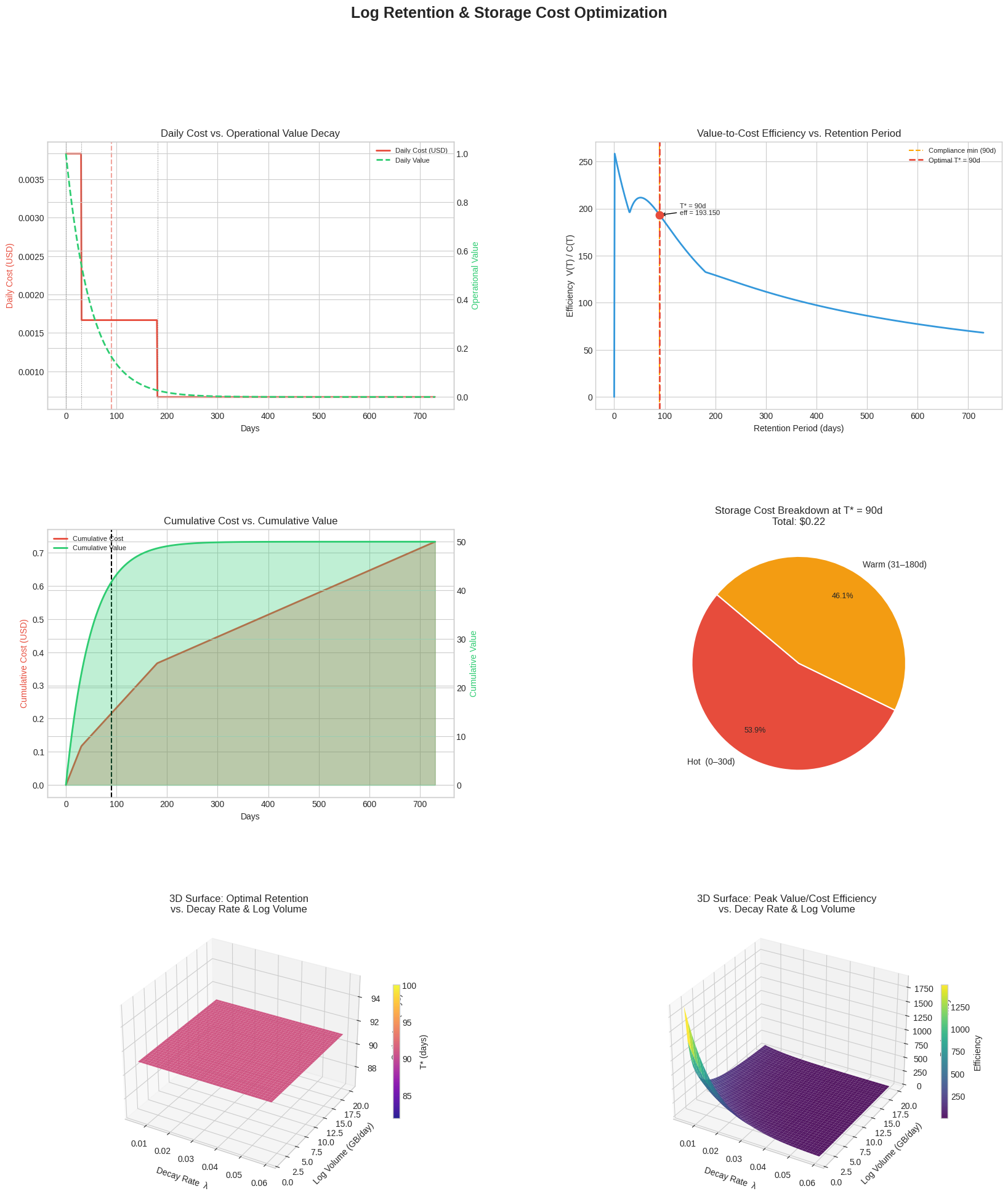
Figure saved as log_retention_optimization.png
Key Takeaways
The math confirms what intuition suggests but makes it quantitative:
$$T^* = \arg\max_{T \geq T_{\min}} \frac{\int_0^T V_0 e^{-\lambda t},dt}{\int_0^T r(t)\cdot p(t),dt}$$
Once you parameterize $\lambda$ from your own access logs (how often do engineers actually open a 90-day-old log?) and plug in real storage pricing, this framework gives you a defensible, data-driven retention policy — not just a round number someone picked years ago.