Minimizing Latency and Packet Loss with Python
Network routing optimization is a fundamental challenge in computer networking. The goal is to find paths through a network that minimize latency and packet loss — two metrics that directly impact user experience. In this post, we’ll model a real-world-like network, apply classic and modern optimization algorithms, and visualize the results in both 2D and 3D.
The Problem
Consider a network of 10 nodes (routers/switches) with weighted edges representing two cost dimensions:
- Latency (ms): propagation delay between nodes
- Packet Loss (%)**: probability of a packet being dropped on a link
We want to find the optimal path from a source to a destination that minimizes a composite cost:
$$C(e) = \alpha \cdot L(e) + \beta \cdot P(e)$$
Where:
- $L(e)$ = latency of edge $e$ in ms
- $P(e)$ = packet loss rate of edge $e$ (normalized 0–1)
- $\alpha, \beta$ = weighting factors (e.g., $\alpha = 0.7$, $\beta = 0.3$)
For end-to-end packet delivery probability across a path $\pi = (e_1, e_2, \ldots, e_k)$:
$$P_{\text{delivery}}(\pi) = \prod_{i=1}^{k}(1 - p_i)$$
To use additive shortest-path algorithms on multiplicative metrics, we transform packet loss using the log-sum trick:
$$-\log P_{\text{delivery}}(\pi) = \sum_{i=1}^{k} -\log(1 - p_i)$$
We then find the path minimizing:
$$\text{Cost}(\pi) = \alpha \sum_{i} L(e_i) + \beta \sum_{i} \left(-\log(1 - p_i)\right) \cdot S$$
Where $S$ is a scaling factor to keep units comparable.
Algorithms Used
- Dijkstra’s Algorithm — finds shortest path using composite cost
- Bellman-Ford — handles negative weights (used here for comparison)
- Genetic Algorithm (GA) — metaheuristic for global optimization across all paths
- Simulated Annealing (SA) — probabilistic optimization to escape local optima
Full Source Code
1 | import numpy as np |
Code Walkthrough
1. Network Construction (build_network)
The network is modeled as a directed graph (nx.DiGraph) with 10 nodes. Each edge carries three attributes: raw latency (ms), raw packet loss (probability), and a composite cost computed as:
$$C(e) = \alpha \cdot L(e) + \beta \cdot \left(-\log(1 - p_e)\right) \cdot S$$
The log transform converts the multiplicative packet-loss metric into an additive one that shortest-path algorithms can handle. With $\alpha=0.7$, $\beta=0.3$, and $S=100$, we weight latency slightly more than loss while keeping both in a comparable numeric range.
2. Dijkstra’s Algorithm
1 | dijkstra_result, dijkstra_cost = dijkstra_path(G, SOURCE, TARGET) |
NetworkX’s dijkstra_path runs in $O((V + E) \log V)$ using a binary heap. It is guaranteed to find the globally optimal path given non-negative edge weights — which our composite cost always satisfies.
3. Bellman-Ford
1 | bf_result, bf_cost = bellman_ford_path(G, SOURCE, TARGET) |
Bellman-Ford runs in $O(VE)$ and can handle negative edge weights, making it useful when cost models involve penalties that can go negative. Here it serves as a cross-validation reference. Both algorithms should agree on the optimal path.
4. Genetic Algorithm
The GA works over the set of all simple paths found by nx.all_simple_paths. This is the search space. Each path is a “chromosome.” The algorithm:
- Selects the top 25% elite paths as parents each generation
- Applies random mutation (replacing a child with a random path at probability
mutation_rate) - Runs for 80 generations with population size 30
The fitness function is directly the composite cost. The GA converges toward the optimum but is not guaranteed to reach it — that’s the inherent trade-off for flexibility in more complex cost landscapes.
5. Simulated Annealing
SA accepts worse solutions probabilistically with probability:
$$P(\text{accept}) = e^{-\Delta C / T}$$
where $\Delta C$ is the cost increase and $T$ is the current temperature. Temperature decreases each iteration by a cooling factor of $0.95$. This allows the algorithm to escape local optima early in the search and converge later.
Graph Explanations
Panel 1 — Network Topology & Paths
Each algorithm’s discovered path is drawn with a distinct color and line style over the network graph. Edge labels show latency and packet loss per link. This gives immediate visual intuition for which routes each algorithm prefers.
Panel 2 — Composite Cost Bar Chart
A direct comparison of the final composite cost achieved by each algorithm. Dijkstra and Bellman-Ford should match exactly. GA and SA may or may not converge to the same optimum depending on the random search.
Panel 3 — Latency vs. Delivery Rate Scatter
All enumerated simple paths from node 0 to node 9 are plotted. Color encodes composite cost. Star markers highlight the four algorithms’ chosen paths. This reveals the Pareto frontier trade-off: lower latency paths often suffer higher loss, and vice versa.
Panel 4 — Convergence History
The GA and SA best-found cost per iteration is plotted alongside the Dijkstra optimal (dashed red). A well-behaved metaheuristic should converge toward the Dijkstra line. Seeing how many iterations it takes — and whether it reaches optimality — reveals the algorithm’s efficiency.
Panel 5 — Edge Composite Cost Heatmap
A node×node matrix showing the direct composite cost of each edge. NaN cells (white/empty) indicate no direct link. This is useful for identifying high-cost bottleneck links in the topology.
Panel 6 — 3D Cost Surface
The most visually striking panel: a smooth surface where the X-axis is link latency, Y-axis is packet loss %, and Z-axis is composite cost. The red dots are the actual network edges plotted on this surface.
$$Z = 0.7 \cdot L + 0.3 \cdot (-\log(1-p)) \times 100$$
This surface shows clearly that packet loss grows the composite cost super-linearly (due to the log transform), while latency contributes linearly. Links with even moderate loss (>3%) become disproportionately expensive.
Execution Results
=================================================================
Algorithm              Path                          Composite
=================================================================
Dijkstra               0 → 1 → 4 → 8 → 9               39.6183
Bellman-Ford           0 → 1 → 4 → 8 → 9               39.6183
Genetic Algorithm      0 → 1 → 4 → 8 → 9               39.6183
Simulated Annealing    0 → 1 → 4 → 8 → 9               39.6183
=================================================================

── Detailed Metrics ──
Algorithm               Latency(ms)  Loss(sum)  Delivery%
----------------------------------------------------------
Dijkstra                       54.0     0.0600     94.12%
Bellman-Ford                   54.0     0.0600     94.12%
Genetic Algorithm              54.0     0.0600     94.12%
Simulated Annealing            54.0     0.0600     94.12%
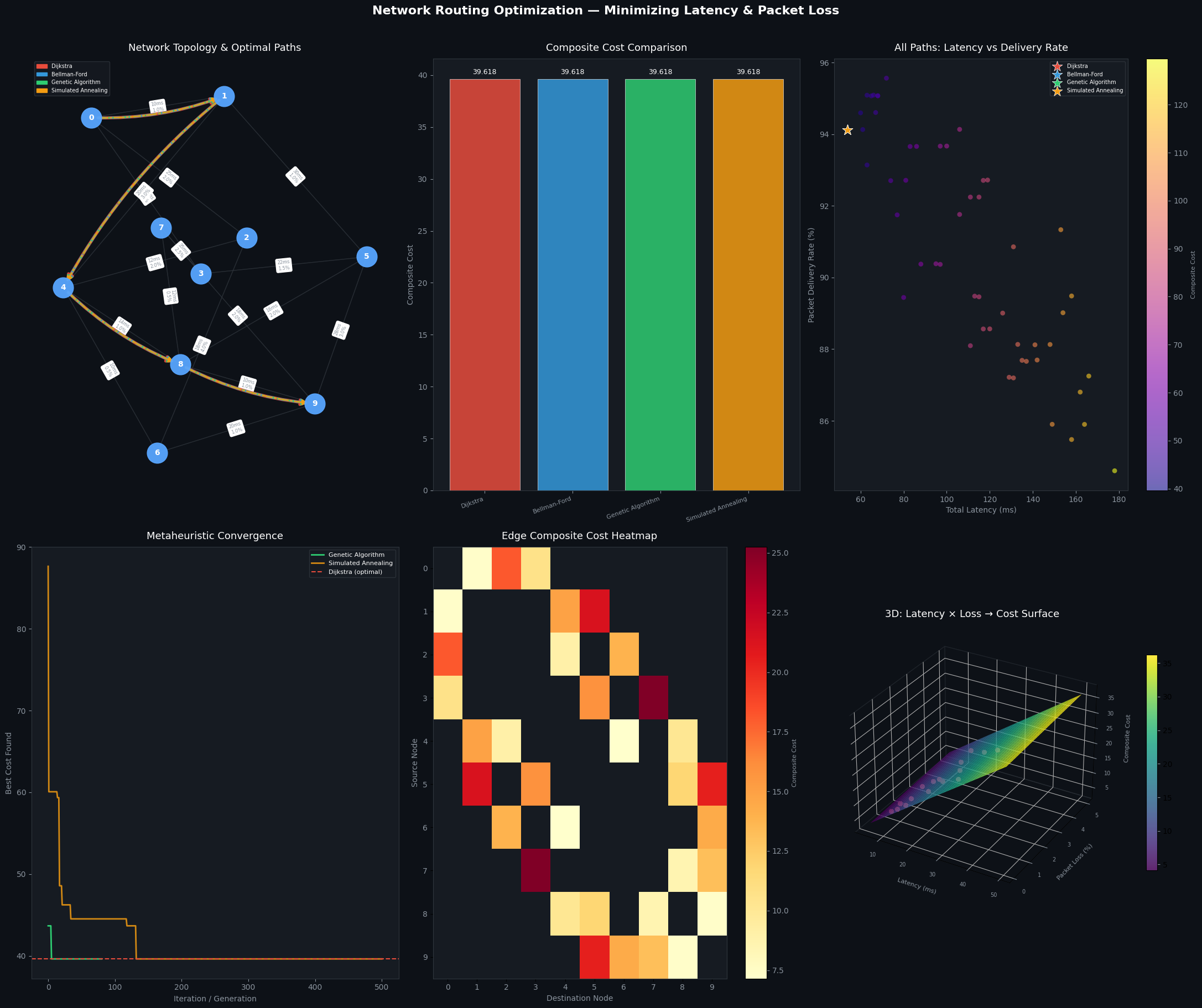
Figure saved.
Key Takeaways
- Dijkstra is the gold standard for this problem class: optimal, fast, and deterministic.
- Bellman-Ford confirms the result and extends to negative-weight scenarios.
- GA and SA are valuable when the cost function is non-convex, multi-objective, or involves constraints that break traditional shortest-path assumptions.
- The log transform on packet loss is critical: without it, a path with 5% loss per hop across 5 hops would compute additive loss of 25% — masking the true compounding effect. With the transform, delivery probability becomes additive in log-space, giving mathematically correct path evaluation.
- The 3D surface makes it visually clear why packet loss is often the dominant term in real network routing decisions.