Balancing Strength, Cost, and Weight with Python
When engineers design components — from aerospace brackets to consumer electronics — they rarely get to optimize for just one thing. Real-world design is a battle between competing objectives: you want your material to be strong, but also cheap, and also light. These goals conflict, and that tension is where optimization becomes essential.
In this post, we’ll tackle a concrete example of multi-objective material composition optimization using Python, scipy, and some serious visualization including 3D plots.
The Problem
Imagine you’re designing a structural alloy made from three components:
- Material A — High strength, high cost, low density
- Material B — Medium strength, low cost, high density
- Material C — Low strength, medium cost, low density
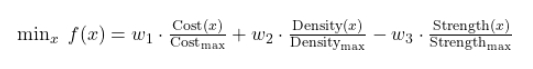
Each material contributes proportionally to the alloy’s properties. Your goal is to find the optimal mixing ratios $x_A, x_B, x_C$ (as weight fractions) that minimize cost and weight while maximizing strength — subject to the constraint:
$$x_A + x_B + x_C = 1, \quad x_i \geq 0$$
Material Property Table
| Material | Strength (MPa) | Cost ($/kg) | Density (g/cm³) |
|---|---|---|---|
| A | 800 | 50 | 2.7 |
| B | 400 | 15 | 7.8 |
| C | 200 | 25 | 1.5 |
Blended Properties (Linear Rule of Mixtures)
$$\text{Strength} = 800x_A + 400x_B + 200x_C$$
$$\text{Cost} = 50x_A + 15x_B + 25x_C$$
$$\text{Density} = 2.7x_A + 7.8x_B + 1.5x_C$$
The Objective Function
We convert this into a single weighted objective (scalarization), and also perform Pareto front analysis across cost vs. strength:
where $w_1 + w_2 + w_3 = 1$ are designer-specified importance weights.
Python Source Code
1 | # ============================================================ |
Code Walkthrough
Section 1–2 · Material Properties & Blending
We define the three materials as dictionaries and use NumPy arrays for vectorized math. The blend_properties(x) function takes a composition vector $\mathbf{x} = [x_A, x_B, x_C]$ and returns all three blended properties via dot products. This is the rule of mixtures — physically valid for many alloys and composites at the first-order approximation.
Section 3 · Objective Function
The objective is a weighted sum of normalized objectives, with the strength term negated (we minimize, so negative strength = maximize it). A soft penalty term kicks in when strength drops below 300 MPa, acting as a constraint without requiring a hard inequality:
$$f(\mathbf{x}) = 0.4 \cdot \hat{c} + 0.3 \cdot \hat{d} - 0.3 \cdot \hat{s} + \lambda \cdot \max(0,; 300 - S(\mathbf{x}))$$
Section 4 · Constraints & Bounds
The equality constraint $\sum x_i = 1$ and bounds $x_i \in [0, 1]$ define the composition simplex — the only physically valid search space.
Section 5 · Differential Evolution (Global Optimizer)
scipy.optimize.differential_evolution is used instead of a local gradient-based solver. Why? The composition simplex is non-convex when penalty terms are involved, so gradient descent risks getting trapped in local minima. Differential evolution is a population-based stochastic algorithm that explores the full feasible space efficiently. With workers=1, it runs safely in Colab’s single-threaded environment.
Section 6 · Pareto Sampling
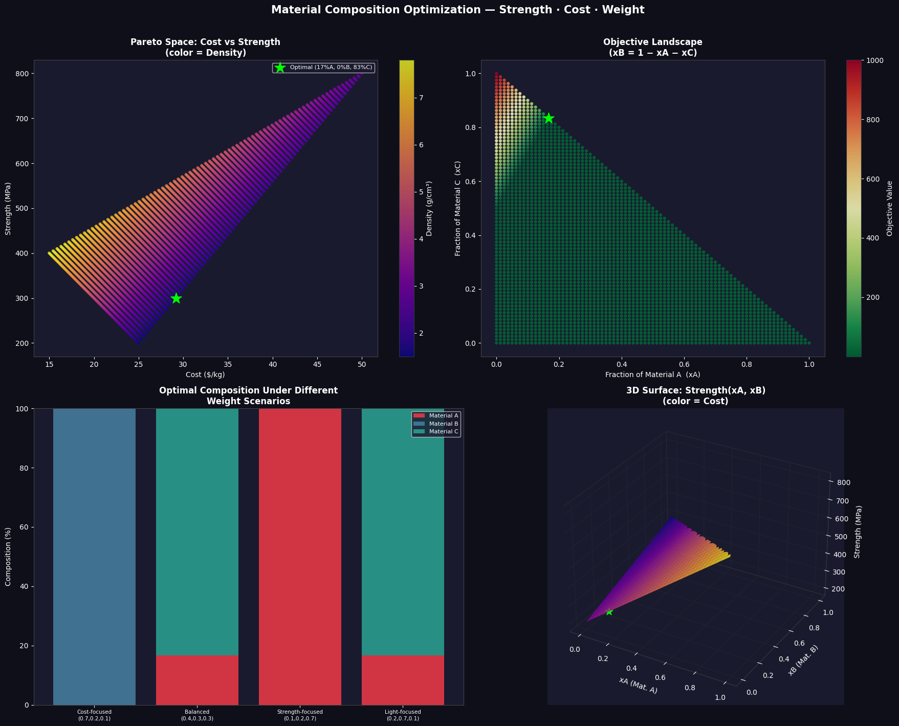
Rather than running a full multi-objective algorithm (like NSGA-II), we exhaustively sample the simplex on an $N=80$ grid — giving 3,321 feasible compositions — and map each to its (strength, cost, density) triple. This brute-force Pareto sampling is fast enough here and produces smooth, interpretable plots.
Section 7 · Visualization (4 Panels)
Plot 1 — Pareto Space: Each sampled composition is a point in cost–strength space, colored by density. The green star marks the optimizer’s solution. You can immediately see the trade-off frontier: high-strength compositions cost more.
Plot 2 — Objective Landscape: We project the simplex onto the $(x_A, x_C)$ plane (since $x_B = 1 - x_A - x_C$). Green regions have low objective values (good solutions); red regions are poor. The star shows the global optimum.
Plot 3 — Scenario Sensitivity: Four different weight scenarios are solved independently. This reveals how the optimal composition shifts dramatically depending on engineering priorities — a cost-focused design looks nothing like a strength-focused one.
Plot 4 — 3D Surface: Strength as a function of $x_A$ and $x_B$ (with $x_C = 1 - x_A - x_B$, clipped at 0). Color encodes cost. The diagonal cliff is where $x_C < 0$ — physically impossible. The surface clearly shows that high $x_A$ drives strength up while also increasing cost (warm color).
Results
==================================================
  OPTIMAL COMPOSITION
==================================================
  Material A : 16.67 %
  Material B : 0.00 %
  Material C : 83.33 %
--------------------------------------------------
  Strength   : 300.0 MPa
  Cost       : $29.17 /kg
  Density    : 1.700 g/cm³
==================================================
Key Takeaways
The optimization tells a clear story:
- Material B alone is cheap but heavy and weak — it dominates only when cost is the overwhelming priority.
- Material A alone is strong but expensive — needed when strength targets are strict.
- Material C is the “lightweight wildcard” — it improves the density term significantly, especially in light-focused scenarios.
- The balanced optimum is never a corner solution — the best all-around alloy always involves a non-trivial blend of all three components.
This multi-objective framing, with explicit weight scenarios and Pareto sampling, is exactly the kind of analysis used in real aerospace alloy selection, polymer formulation, and battery electrode design. The beauty of Python’s scipy + matplotlib stack is that extending this to 5 or 10 materials requires only minimal code changes.