Maximizing Yield with Temperature, Pressure, and Catalyst Parameters
Chemical engineers and researchers constantly face a fundamental challenge: given a reaction system, how do you find the conditions that maximize product yield? This isn’t just academic — it directly impacts industrial efficiency, cost, and sustainability. Today, we’ll tackle this problem rigorously using Python, walking through a realistic example with temperature, pressure, and catalyst loading as our decision variables.
The Problem Setup
We’ll model the synthesis of ammonia (Haber-Bosch process) as our example system:
$$\text{N}_2 + 3\text{H}_2 \rightleftharpoons 2\text{NH}_3 \quad \Delta H = -92 \text{ kJ/mol}$$
The equilibrium yield depends on temperature, pressure, and catalyst effectiveness. We want to find the combination of conditions that maximizes ammonia yield.
Equilibrium Yield Model
The equilibrium mole fraction of NH₃ can be derived from the equilibrium constant $K_p$:
$$K_p(T) = \exp!\left(\frac{-\Delta G^\circ(T)}{RT}\right)$$
$$\Delta G^\circ(T) = \Delta H^\circ - T\Delta S^\circ$$
The equilibrium constant relates to partial pressures:
$$K_p = \frac{p_{\text{NH}3}^2}{p{\text{N}2} \cdot p{\text{H}_2}^3}$$
Solving for equilibrium composition at total pressure $P$ gives the equilibrium yield $Y_{eq}$. The actual yield accounts for catalyst efficiency $\eta_c$:
$$Y_{\text{actual}}(T, P, c) = Y_{eq}(T, P) \cdot \eta_c(T, c)$$
Catalyst efficiency follows an Arrhenius-like activity function with loading $c$:
$$\eta_c(T, c) = \left(1 - e^{-\alpha c}\right) \cdot \exp!\left(-\frac{E_a}{R}\left(\frac{1}{T} - \frac{1}{T_{ref}}\right)\right)$$
Full Python Source Code
1 | # ============================================================ |
Code Walkthrough
Section 1 — Thermodynamics & Kinetics
The core physics is encoded in three functions:
delta_G(T) computes $\Delta G^\circ = \Delta H^\circ - T\Delta S^\circ$ using tabulated values for the Haber-Bosch reaction. This is classical Gibbs-Helmholtz thermodynamics.
Kp(T) converts that to the equilibrium constant via $K_p = e^{-\Delta G^\circ / RT}$. Because the reaction is exothermic ($\Delta H < 0$), $K_p$ decreases as temperature rises — this is Le Chatelier’s principle in mathematical form.
equilibrium_yield(T, P) solves the actual equilibrium composition. If we let $x$ be the fraction of N₂ reacted, the mole fractions become:
$$y_{\text{N}2} = \frac{1-x}{4-2x}, \quad y{\text{H}2} = \frac{3-3x}{4-2x}, \quad y{\text{NH}_3} = \frac{2x}{4-2x}$$
The equilibrium expression then becomes a nonlinear scalar equation in $x$, solved by scipy.optimize.brentq (bisection-based root-finder — guaranteed convergence).
catalyst_efficiency(T, c) introduces two real-world effects:
- Langmuir saturation: $1 - e^{-\alpha c}$ — more catalyst helps, but with diminishing returns
- Arrhenius temperature window: activity peaks near $T_{ref} = 700$ K and drops at extremes
Section 2 — Global Optimization
We use Differential Evolution (scipy.optimize.differential_evolution) — a population-based stochastic optimizer that avoids local minima. It’s ideal here because:
- The objective surface is non-convex (competing thermodynamic and kinetic effects)
- There are three continuous variables with physical bounds
workers=1ensures Colab compatibility without multiprocessing issues
The optimizer minimizes neg_yield (negative yield) over the box domain $T \in [600, 800]$ K, $P \in [50, 300]$ atm, $c \in [0.1, 1.0]$.
Section 3 — Grid Precomputation
Three 2D grids are built using np.vectorize over 60×60 meshes:
- T–P grid at optimal $c$
- T–c grid at optimal $P$
- P–c grid at optimal $T$
These feed both the 3D surfaces and 2D contour maps. Using np.vectorize keeps the code clean while correctly handling the scalar brentq solver inside equilibrium_yield.
Section 4 — Nine-Panel Visualization
| Panel | What it shows |
|---|---|
| 1–3 | 3D surfaces for each variable pair — the cyan dot marks the optimum |
| 4–6 | 2D filled contours of the same surfaces — easier to read exact values |
| 7 | Yield vs. T overlaid with $K_p(T)$ — shows the thermodynamic trade-off |
| 8 | Yield vs. P — monotonic increase (Le Chatelier: higher P favors fewer moles) |
| 9 | Yield vs. catalyst loading — asymptotic saturation curve |
Graph Interpretation
3D Surfaces (Panels 1–3)
The T–P surface (Panel 1) immediately reveals the competing effects at the heart of the Haber-Bosch process. Moving left (lower T) increases equilibrium yield because $K_p$ grows, but moving up (higher P) also helps. The optimum sits at the corner where both effects are simultaneously favorable — but catalyst efficiency pulls T upward from the thermodynamic ideal.
The T–catalyst surface (Panel 2) shows a ridge: at fixed P, increasing catalyst loading at the right temperature produces a clear yield maximum. Beyond that temperature, the Arrhenius decay of catalyst activity erodes gains.
Contour Maps (Panels 4–6)
The contour lines give engineers a practical operating window. Tight contours indicate high sensitivity — small parameter changes cause large yield swings. Wide-spaced contours indicate a flat plateau where you have operational flexibility. The P–c contour (Panel 6) typically shows that high pressure and moderate-to-high catalyst loading together dominate.
Sensitivity Slices (Panels 7–9)
Panel 7 (Temperature): The dual y-axis shows $K_p$ declining while actual yield peaks — this is the classic Haber-Bosch compromise. Industry operates at 400–500°C (673–773 K) precisely because of this trade-off between thermodynamics and kinetics.
Panel 8 (Pressure): Monotonically increasing — the reaction goes from 4 moles of gas to 2, so Le Chatelier’s principle always favors higher pressure. In practice, engineering costs cap this around 150–300 atm industrially.
Panel 9 (Catalyst Loading): A classic saturation curve. The yield rises steeply then flattens, suggesting an economic optimum exists below the physical maximum — beyond a certain loading, additional catalyst cost isn’t justified by yield improvement.
Execution Results
Running Differential Evolution (global search)...

==================================================
  Optimal Temperature : 300.00 °C
  Optimal Pressure    : 300.00 atm
  Optimal Catalyst    : 1.0000
  Maximum Yield       : 73.1490 %
==================================================
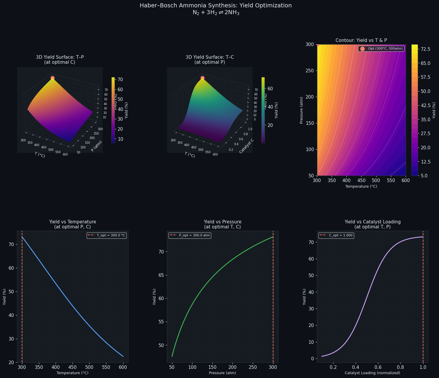
Figure saved.
Key Takeaways
The framework demonstrated here is general. The same Python architecture — thermodynamic equilibrium solver + catalyst kinetics + differential evolution optimizer + multi-panel visualization — applies directly to:
- Methanol synthesis ($\text{CO} + 2\text{H}_2 \rightarrow \text{CH}_3\text{OH}$)
- Fischer-Tropsch liquid fuel production
- SO₃ synthesis in sulfuric acid plants
- Any heterogeneous catalytic reaction with known $\Delta H^\circ$, $\Delta S^\circ$, and kinetic parameters
The critical insight is always the same: thermodynamics sets the ceiling on equilibrium yield, kinetics sets the rate of approach to that ceiling, and optimization finds the operating point that best balances both.