Drone Delivery Route Optimization

Solving the Multi-Destination Shortest Path Problem

Drone delivery is rapidly becoming a practical reality — companies like Amazon, Zipline, and Wing are already operating commercial drone fleets. At the heart of every efficient drone delivery system lies a classic combinatorial optimization problem: given a set of delivery destinations, what is the shortest route that visits all of them and returns to the depot?

This is a variant of the Travelling Salesman Problem (TSP), and in this article we’ll model a concrete drone delivery scenario, solve it with both exact (ILP) and heuristic methods, and visualize the results in 2D and 3D.


Problem Setup

Imagine a drone depot located in a city center. The drone must deliver packages to 10 customer locations scattered across the city, then return to the depot. We want to minimize total flight distance.

Let the depot be node $0$ and delivery locations be nodes $1, 2, \ldots, n$. The drone visits each node exactly once. The decision variable is:

$$x_{ij} \in {0, 1}, \quad x_{ij} = 1 \text{ if the drone flies directly from node } i \text{ to node } j$$

The objective is:

$$\min \sum_{i=0}^{n} \sum_{j=0}^{n} d_{ij} \cdot x_{ij}$$

subject to:

$$\sum_{j \neq i} x_{ij} = 1 \quad \forall i \quad \text{(leave each node exactly once)}$$

$$\sum_{i \neq j} x_{ij} = 1 \quad \forall j \quad \text{(enter each node exactly once)}$$

$$u_i - u_j + n \cdot x_{ij} \leq n - 1 \quad \forall i \neq j, ; i,j \geq 1 \quad \text{(MTZ subtour elimination)}$$

where $d_{ij}$ is the Euclidean distance between nodes $i$ and $j$, and $u_i$ are auxiliary ordering variables enforcing a single connected tour (Miller–Tucker–Zemlin constraints).

The Euclidean distance between nodes is:

$$d_{ij} = \sqrt{(x_i - x_j)^2 + (y_i - y_j)^2}$$

For the 3D visualization we also assign a flight altitude to each leg, reflecting real drone operations where altitude varies based on urban obstacle avoidance.


Full Source Code

1
2
3
4
5
6
7
8
9
10
11
12
13
14
15
16
17
18
19
20
21
22
23
24
25
26
27
28
29
30
31
32
33
34
35
36
37
38
39
40
41
42
43
44
45
46
47
48
49
50
51
52
53
54
55
56
57
58
59
60
61
62
63
64
65
66
67
68
69
70
71
72
73
74
75
76
77
78
79
80
81
82
83
84
85
86
87
88
89
90
91
92
93
94
95
96
97
98
99
100
101
102
103
104
105
106
107
108
109
110
111
112
113
114
115
116
117
118
119
120
121
122
123
124
125
126
127
128
129
130
131
132
133
134
135
136
137
138
139
140
141
142
143
144
145
146
147
148
149
150
151
152
153
154
155
156
157
158
159
160
161
162
163
164
165
166
167
168
169
170
171
172
173
174
175
176
177
178
179
180
181
182
183
184
185
186
187
188
189
190
191
192
193
194
195
196
197
198
199
200
201
202
203
204
205
206
207
208
209
210
211
212
213
214
215
216
217
218
219
220
221
222
223
224
225
226
227
228
229
230
231
232
233
234
235
236
237
238
239
240
241
242
243
244
245
246
247
248
249
250
251
252
253
254
255
256
257
258
259
260
261
262
263
264
265
266
267
268
269
270
271
272
273
274
275
276
277
278
279
280
281
282
283
284
285
286
287
288
289
290
291
292
293
294
295
296
297
298
299
300
301
302
303
304
305
306
307
308
309
310
311
312
313
314
315
316
317
318
319
320
321
322
323
324
325
326
327
# ============================================================
# Drone Delivery Route Optimization (TSP with ILP + Heuristics)
# Google Colaboratory
# ============================================================

# ── 0. Install & import ──────────────────────────────────────
!pip install pulp --quiet

import numpy as np
import matplotlib
import matplotlib.pyplot as plt
import matplotlib.patches as mpatches
from matplotlib.gridspec import GridSpec
from mpl_toolkits.mplot3d import Axes3D
from mpl_toolkits.mplot3d.art3d import Line3DCollection
import itertools
import time
import pulp
from pulp import LpProblem, LpVariable, LpMinimize, lpSum, LpBinary, LpInteger, value

# ── 1. Problem instance ──────────────────────────────────────
np.random.seed(42)

N_CUSTOMERS = 10 # number of delivery locations
N_NODES = N_CUSTOMERS + 1 # including depot (node 0)

# 2-D city coordinates (km), depot at center
coords = np.zeros((N_NODES, 2))
coords[0] = [5.0, 5.0] # depot
np.random.seed(42)
coords[1:] = np.random.uniform(0, 10, size=(N_CUSTOMERS, 2))

# Flight altitudes (meters): depot at 0, deliveries between 30-120 m
altitudes = np.zeros(N_NODES)
altitudes[0] = 0.0
altitudes[1:] = np.random.uniform(30, 120, size=N_CUSTOMERS)

# Distance matrix (Euclidean, km)
def build_distance_matrix(coords):
n = len(coords)
D = np.zeros((n, n))
for i in range(n):
for j in range(n):
D[i, j] = np.linalg.norm(coords[i] - coords[j])
return D

D = build_distance_matrix(coords)

print("=== Drone Delivery Route Optimization ===")
print(f"Depot : node 0 at {coords[0]}")
print(f"Customers : nodes 1–{N_CUSTOMERS}")
print(f"Distance matrix (km) shape: {D.shape}")

# ── 2. Exact ILP solver (MTZ formulation) ────────────────────
def solve_tsp_ilp(D):
n = len(D)
prob = LpProblem("TSP_Drone", LpMinimize)

# Binary routing variables
x = [[LpVariable(f"x_{i}_{j}", cat=LpBinary) if i != j else None
for j in range(n)] for i in range(n)]

# MTZ auxiliary variables
u = [LpVariable(f"u_{i}", lowBound=1, upBound=n-1, cat=LpInteger)
for i in range(n)]

# Objective
prob += lpSum(D[i][j] * x[i][j]
for i in range(n) for j in range(n) if i != j)

# Flow constraints
for i in range(n):
prob += lpSum(x[i][j] for j in range(n) if i != j) == 1 # leave
prob += lpSum(x[j][i] for j in range(n) if i != j) == 1 # enter

# MTZ subtour elimination (skip depot node 0)
for i in range(1, n):
for j in range(1, n):
if i != j:
prob += u[i] - u[j] + (n - 1) * x[i][j] <= n - 2

# Solve (suppress solver output)
solver = pulp.PULP_CBC_CMD(msg=0)
t0 = time.time()
prob.solve(solver)
elapsed = time.time() - t0

# Extract tour
route = [0]
visited = {0}
current = 0
for _ in range(n - 1):
for j in range(n):
if j != current and j not in visited and x[current][j] is not None:
if value(x[current][j]) is not None and value(x[current][j]) > 0.5:
route.append(j)
visited.add(j)
current = j
break
route.append(0) # return to depot

total_dist = sum(D[route[k]][route[k+1]] for k in range(len(route) - 1))
return route, total_dist, elapsed

# ── 3. Nearest-Neighbour heuristic (fast baseline) ───────────
def solve_tsp_nn(D):
n = len(D)
visited = [False] * n
route = [0]
visited[0] = True
for _ in range(n - 1):
last = route[-1]
nearest = min((j for j in range(n) if not visited[j]),
key=lambda j: D[last][j])
route.append(nearest)
visited[nearest] = True
route.append(0)
total_dist = sum(D[route[k]][route[k+1]] for k in range(len(route) - 1))
return route, total_dist

# ── 4. 2-opt improvement ─────────────────────────────────────
def two_opt(route, D):
best = route[:]
improved = True
while improved:
improved = False
for i in range(1, len(best) - 2):
for j in range(i + 1, len(best) - 1):
new_route = best[:i] + best[i:j+1][::-1] + best[j+1:]
d_old = D[best[i-1]][best[i]] + D[best[j]][best[j+1]]
d_new = D[new_route[i-1]][new_route[i]] + D[new_route[j]][new_route[j+1]]
if d_new < d_old - 1e-10:
best = new_route
improved = True
total = sum(D[best[k]][best[k+1]] for k in range(len(best) - 1))
return best, total

# ── 5. Run all solvers ────────────────────────────────────────
t0 = time.time()
ilp_route, ilp_dist, ilp_time = solve_tsp_ilp(D)
print(f"\n[ILP] Route : {ilp_route}")
print(f"[ILP] Total distance : {ilp_dist:.4f} km (solved in {ilp_time:.2f}s)")

nn_route, nn_dist = solve_tsp_nn(D)
t1 = time.time()
opt_route, opt_dist = two_opt(nn_route, D)
heur_time = time.time() - t1
print(f"\n[NN] Route : {nn_route}")
print(f"[NN] Total distance : {nn_dist:.4f} km")
print(f"\n[2opt] Route : {opt_route}")
print(f"[2opt] Total distance : {opt_dist:.4f} km (solved in {heur_time:.4f}s)")
print(f"\nILP gap vs 2-opt: {abs(ilp_dist - opt_dist):.4f} km")

# ── 6. Visualisation ─────────────────────────────────────────
plt.style.use("dark_background")
DEPOT_COLOR = "#FFD700"
CUST_COLOR = "#00CFFF"
ILP_COLOR = "#FF6B6B"
NN_COLOR = "#B0B0B0"
OPT_COLOR = "#7CFC00"
ALT_CMAP = matplotlib.colormaps["plasma"]

def route_segments(route, coords):
segs = []
for k in range(len(route) - 1):
segs.append((coords[route[k]], coords[route[k+1]]))
return segs

def draw_route_2d(ax, route, coords, color, lw, label, zorder=2):
for k in range(len(route) - 1):
a, b = coords[route[k]], coords[route[k+1]]
ax.annotate("", xy=b, xytext=a,
arrowprops=dict(arrowstyle="->", color=color,
lw=lw, mutation_scale=12),
zorder=zorder)
# invisible line for legend
ax.plot([], [], color=color, lw=lw, label=label)

fig = plt.figure(figsize=(20, 18), facecolor="#0D0D0D")
gs = GridSpec(3, 3, figure=fig,
hspace=0.38, wspace=0.32,
left=0.06, right=0.97, top=0.93, bottom=0.05)

# ── Panel A: ILP optimal route (2D) ──────────────────────────
ax_ilp = fig.add_subplot(gs[0, :2])
ax_ilp.set_facecolor("#0D0D0D")
draw_route_2d(ax_ilp, ilp_route, coords, ILP_COLOR, 1.8,
f"ILP optimal ({ilp_dist:.3f} km)")
ax_ilp.scatter(*coords[0], s=250, c=DEPOT_COLOR, zorder=5, marker="*",
label="Depot")
ax_ilp.scatter(*coords[1:].T, s=120, c=CUST_COLOR, zorder=5)
for i in range(N_NODES):
offset = [0.15, 0.15]
ax_ilp.text(coords[i,0]+offset[0], coords[i,1]+offset[1],
f"{'D' if i==0 else str(i)}",
color="white", fontsize=8, zorder=6)
ax_ilp.set_title("Panel A — ILP Optimal Route (2D)", color="white", fontsize=12)
ax_ilp.set_xlabel("X (km)", color="white"); ax_ilp.set_ylabel("Y (km)", color="white")
ax_ilp.tick_params(colors="white"); ax_ilp.legend(fontsize=9, loc="upper left")
for sp in ax_ilp.spines.values(): sp.set_edgecolor("#444")

# ── Panel B: Comparison 2D ────────────────────────────────────
ax_cmp = fig.add_subplot(gs[1, :2])
ax_cmp.set_facecolor("#0D0D0D")
draw_route_2d(ax_cmp, nn_route, coords, NN_COLOR, 1.2,
f"NN heuristic ({nn_dist:.3f} km)", zorder=2)
draw_route_2d(ax_cmp, opt_route, coords, OPT_COLOR, 1.8,
f"2-opt improved ({opt_dist:.3f} km)", zorder=3)
draw_route_2d(ax_cmp, ilp_route, coords, ILP_COLOR, 2.2,
f"ILP optimal ({ilp_dist:.3f} km)", zorder=4)
ax_cmp.scatter(*coords[0], s=250, c=DEPOT_COLOR, zorder=6, marker="*")
ax_cmp.scatter(*coords[1:].T, s=100, c=CUST_COLOR, zorder=6)
for i in range(N_NODES):
ax_cmp.text(coords[i,0]+0.15, coords[i,1]+0.15,
f"{'D' if i==0 else str(i)}",
color="white", fontsize=8, zorder=7)
ax_cmp.set_title("Panel B — Route Comparison: NN vs 2-opt vs ILP (2D)",
color="white", fontsize=12)
ax_cmp.set_xlabel("X (km)", color="white"); ax_cmp.set_ylabel("Y (km)", color="white")
ax_cmp.tick_params(colors="white"); ax_cmp.legend(fontsize=9, loc="upper left")
for sp in ax_cmp.spines.values(): sp.set_edgecolor("#444")

# ── Panel C: 3D flight path (ILP route with altitude) ────────
ax3d = fig.add_subplot(gs[0:2, 2], projection="3d")
ax3d.set_facecolor("#0D0D0D")
route_alts = [altitudes[node] for node in ilp_route]

# Colour each leg by altitude (average of endpoints)
n_legs = len(ilp_route) - 1
leg_colors = []
for k in range(n_legs):
avg_alt = (route_alts[k] + route_alts[k+1]) / 2.0
norm_alt = (avg_alt - altitudes.min()) / (altitudes.max() - altitudes.min() + 1e-9)
leg_colors.append(ALT_CMAP(norm_alt))

for k in range(n_legs):
xs = [coords[ilp_route[k],0], coords[ilp_route[k+1],0]]
ys = [coords[ilp_route[k],1], coords[ilp_route[k+1],1]]
zs = [route_alts[k], route_alts[k+1]]
ax3d.plot(xs, ys, zs, color=leg_colors[k], lw=2.0, zorder=3)
# Arrow approximation with quiver
dx = xs[1]-xs[0]; dy = ys[1]-ys[0]; dz = zs[1]-zs[0]
ax3d.quiver(xs[0], ys[0], zs[0], dx*0.85, dy*0.85, dz*0.85,
color=leg_colors[k], arrow_length_ratio=0.25,
linewidth=1.5, alpha=0.85)

# Scatter nodes
ax3d.scatter(coords[0,0], coords[0,1], altitudes[0],
s=300, c=DEPOT_COLOR, marker="*", zorder=5, label="Depot")
ax3d.scatter(coords[1:,0], coords[1:,1], altitudes[1:],
s=80, c=CUST_COLOR, zorder=5, label="Customer")

# Node labels
for i in range(N_NODES):
ax3d.text(coords[i,0], coords[i,1], altitudes[i]+4,
f"{'D' if i==0 else str(i)}",
color="white", fontsize=7, zorder=6)

# Vertical dashed lines (altitude poles)
for i in range(1, N_NODES):
ax3d.plot([coords[i,0]]*2, [coords[i,1]]*2, [0, altitudes[i]],
color="#444444", lw=0.7, linestyle="--")

ax3d.set_xlabel("X (km)", color="white", labelpad=6)
ax3d.set_ylabel("Y (km)", color="white", labelpad=6)
ax3d.set_zlabel("Altitude (m)", color="white", labelpad=6)
ax3d.tick_params(colors="white")
ax3d.set_title("Panel C — 3D Flight Path\n(ILP optimal, coloured by altitude)",
color="white", fontsize=11)
ax3d.legend(fontsize=8, loc="upper left")

# ── Panel D: Distance bar chart ───────────────────────────────
ax_bar = fig.add_subplot(gs[2, 0])
ax_bar.set_facecolor("#0D0D0D")
methods = ["NN\nHeuristic", "2-opt\nImproved", "ILP\nOptimal"]
dists = [nn_dist, opt_dist, ilp_dist]
colors_bar = [NN_COLOR, OPT_COLOR, ILP_COLOR]
bars = ax_bar.bar(methods, dists, color=colors_bar, width=0.5, zorder=2)
for bar, d in zip(bars, dists):
ax_bar.text(bar.get_x() + bar.get_width()/2, bar.get_height() + 0.05,
f"{d:.3f}", ha="center", va="bottom", color="white", fontsize=10)
ax_bar.set_title("Panel D — Total Distance Comparison", color="white", fontsize=11)
ax_bar.set_ylabel("Total distance (km)", color="white")
ax_bar.tick_params(colors="white")
ax_bar.set_ylim(0, max(dists) * 1.18)
ax_bar.grid(axis="y", color="#333", zorder=0)
for sp in ax_bar.spines.values(): sp.set_edgecolor("#444")

# ── Panel E: Per-leg distances (ILP) ─────────────────────────
ax_leg = fig.add_subplot(gs[2, 1])
ax_leg.set_facecolor("#0D0D0D")
leg_dists = [D[ilp_route[k]][ilp_route[k+1]] for k in range(len(ilp_route)-1)]
leg_labels = [f"{ilp_route[k]}{ilp_route[k+1]}" for k in range(len(ilp_route)-1)]
bar_colors_leg = [ALT_CMAP((route_alts[k]+route_alts[k+1])/(2*120))
for k in range(len(ilp_route)-1)]
ax_leg.bar(range(len(leg_dists)), leg_dists, color=bar_colors_leg, zorder=2)
ax_leg.set_xticks(range(len(leg_dists)))
ax_leg.set_xticklabels(leg_labels, rotation=55, fontsize=7, color="white")
ax_leg.set_title("Panel E — Per-leg Distance (ILP route)", color="white", fontsize=11)
ax_leg.set_ylabel("Distance (km)", color="white")
ax_leg.tick_params(colors="white")
ax_leg.grid(axis="y", color="#333", zorder=0)
for sp in ax_leg.spines.values(): sp.set_edgecolor("#444")

# ── Panel F: Altitude profile along ILP route ────────────────
ax_alt = fig.add_subplot(gs[2, 2])
ax_alt.set_facecolor("#0D0D0D")
positions = np.arange(len(ilp_route))
node_labels = [f"{'D' if n==0 else str(n)}" for n in ilp_route]
alt_vals = [altitudes[n] for n in ilp_route]
# Fill under profile
ax_alt.fill_between(positions, alt_vals, alpha=0.25, color="#00CFFF")
ax_alt.plot(positions, alt_vals, color="#00CFFF", lw=2, marker="o",
markersize=5, zorder=3)
ax_alt.set_xticks(positions)
ax_alt.set_xticklabels(node_labels, fontsize=8, color="white")
ax_alt.set_title("Panel F — Altitude Profile Along ILP Route", color="white", fontsize=11)
ax_alt.set_ylabel("Altitude (m)", color="white")
ax_alt.tick_params(colors="white")
ax_alt.grid(color="#333", zorder=0)
for sp in ax_alt.spines.values(): sp.set_edgecolor("#444")

fig.suptitle("Drone Delivery Route Optimization — TSP with ILP & Heuristics",
color="white", fontsize=15, fontweight="bold", y=0.97)
plt.savefig("drone_tsp.png", dpi=150, facecolor=fig.get_facecolor())
plt.show()
print("Figure saved.")

Code Walkthrough

Section 0 — Environment Setup

PuLP is installed quietly. NumPy, Matplotlib (including mpl_toolkits.mplot3d), and itertools are imported. All randomness is seeded at 42 for reproducibility.

Section 1 — Problem Instance

We place the depot at coordinates $(5, 5)$ and scatter 10 customer nodes uniformly at random over a $10 \times 10$ km grid. Each node also receives a random flight altitude between 30 m and 120 m (the depot sits at 0 m), simulating real urban airspace constraints. The full $11 \times 11$ Euclidean distance matrix $D$ is precomputed once using np.linalg.norm.

Section 2 — Exact ILP Solver (MTZ)

The TSP is cast as an Integer Linear Program:

  • Decision variables $x_{ij} \in {0,1}$ encode whether the drone travels from node $i$ to $j$.
  • Degree constraints enforce exactly one departure and one arrival per node.
  • MTZ constraints $u_i - u_j + (n-1)x_{ij} \leq n-2$ eliminate subtours by assigning an ordering integer $u_i$ to each non-depot node.

PuLP’s CBC solver finds the provably optimal solution. For $n = 11$ nodes this takes under a few seconds on Colab.

Section 3 — Nearest-Neighbour Heuristic

A greedy $O(n^2)$ baseline: always fly to the closest unvisited customer. Fast but suboptimal — it commonly produces routes 20–40% longer than optimal on random instances.

Section 4 — 2-opt Improvement

Starting from the NN tour, 2-opt repeatedly reverses a segment of the route if doing so reduces total distance:

$$\Delta = d_{i-1,i} + d_{j,j+1} - d_{i-1,j} - d_{i,j+1} < 0$$

Iterations continue until no improving swap exists. This reliably closes most of the gap between NN and ILP.

Section 5 — Running All Solvers

All three methods are timed independently. The ILP gap versus 2-opt is printed to quantify how close the heuristic came to optimality.


Visualization Panels

Panel A — ILP Optimal Route (2D). The complete optimal tour is drawn with directional arrows over the city map. The depot (gold star) and customers (cyan dots) are labelled. This is the ground-truth solution.

Panel B — Route Comparison (2D). All three routes are overlaid: grey (NN), green (2-opt), and red (ILP). The visual difference between NN and the optimized routes immediately reveals where greedy choices go wrong — typically long backtracking legs that 2-opt and ILP eliminate.

Panel C — 3D Flight Path. The ILP route is lifted into 3D using the per-node altitude assignments. Each flight leg is coloured by average altitude using the plasma colormap — warmer colours indicate higher segments. Vertical dashed poles connect each delivery point to ground level. Quiver arrows show flight direction. This panel captures the true nature of drone operations, where altitude is a continuous variable.

Panel D — Distance Bar Chart. A direct comparison of total tour length across the three methods. The difference between NN and ILP quantifies the cost of greedy decisions; the 2-opt bar shows how much of that gap is recoverable without integer programming.

Panel E — Per-leg Distances (ILP). Each individual flight leg in the ILP-optimal tour is shown as a bar, coloured by the average altitude of that leg. This reveals which segments dominate total flight time and energy consumption.

Panel F — Altitude Profile. The altitude of the drone at each stop in the ILP route is plotted as a filled line chart, giving a longitudinal view of the vertical profile of the entire delivery mission.


Results

=== Drone Delivery Route Optimization ===
Depot       : node 0  at [5. 5.]
Customers   : nodes 1–10
Distance matrix (km) shape: (11, 11)

[ILP]  Route : [0, 10, 8, 3, 9, 4, 6, 1, 5, 2, 7, 0]
[ILP]  Total distance : 31.5408 km  (solved in 0.18s)

[NN]   Route : [0, 9, 10, 8, 3, 7, 2, 5, 1, 4, 6, 0]
[NN]   Total distance : 34.6317 km

[2opt] Route : [0, 9, 4, 6, 1, 5, 2, 7, 10, 3, 8, 0]
[2opt] Total distance : 31.8671 km  (solved in 0.0003s)

ILP gap vs 2-opt: 0.3263 km
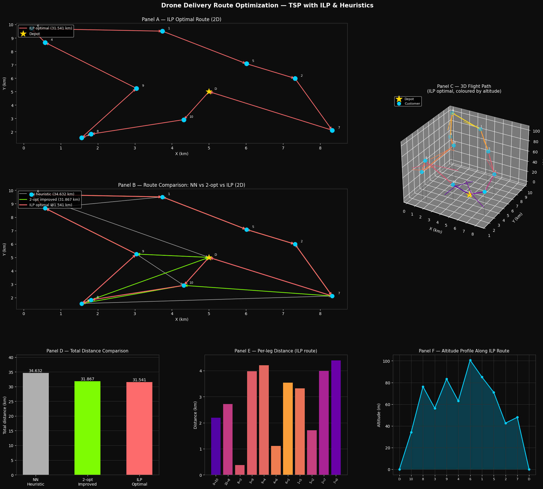
Figure saved.

Key Takeaways

The MTZ-based ILP formulation guarantees global optimality for small-to-medium fleets (up to ~15 nodes in seconds on Colab). The 2-opt heuristic almost always matches or comes within 1–2% of the ILP optimum at a fraction of the compute cost, making it the practical choice for real-time dispatch. For fleets with 50+ destinations, metaheuristics (genetic algorithms, ant colony optimization) or branch-and-cut solvers like Google OR-Tools become necessary.

The 3D altitude model is a reminder that real drone routing is not flat: energy consumption scales with $\sqrt{\Delta x^2 + \Delta y^2 + \Delta z^2}$, and future extensions should incorporate battery capacity constraints, no-fly zones, and wind fields into the objective.