Minimizing Tardiness & Maximizing Utilization
Modern manufacturing and service operations face a fundamental tension: finish jobs on time and keep machines busy. In this post, we tackle both objectives simultaneously using Integer Linear Programming (ILP), visualize the resulting Gantt chart in 3D, and dissect every trade-off the solver finds.
Problem Setup
We have 5 jobs to schedule on 3 machines. Each job must visit all three machines in a fixed order (a classic flow shop). The data:
| Job | Processing Times (M1, M2, M3) | Due Date | Weight |
|---|---|---|---|
| J1 | 4, 2, 3 | 12 | 2 |
| J2 | 3, 5, 2 | 15 | 1 |
| J3 | 2, 3, 4 | 10 | 3 |
| J4 | 5, 1, 3 | 20 | 1 |
| J5 | 1, 4, 2 | 14 | 2 |
Objective (weighted sum, bi-criteria):
$$\min ; \alpha \sum_{j} w_j T_j ;-; (1-\alpha) U$$
where:
- $T_j = \max(C_j - d_j,; 0)$ — tardiness of job $j$
- $C_j$ — completion time of job $j$ on the last machine
- $d_j$ — due date of job $j$
- $w_j$ — weight (priority) of job $j$
- $U$ — overall machine utilization $\in [0,1]$
- $\alpha \in [0,1]$ — trade-off parameter
Decision Variables
$$x_{j,k} \in {0,1}: \text{job } j \text{ is scheduled at position } k$$
$$S_{j,m} \geq 0: \text{start time of job } j \text{ on machine } m$$
Constraints
Permutation constraint (each job assigned to exactly one position, each position filled by exactly one job):
$$\sum_k x_{j,k} = 1 ;\forall j, \qquad \sum_j x_{j,k} = 1 ;\forall k$$
Precedence within a job (machine order must be respected):
$$S_{j,m+1} \geq S_{j,m} + p_{j,m} ;\forall j, m$$
No overlap on each machine (jobs at consecutive positions cannot overlap):
$$S_{\sigma(k+1),m} \geq S_{\sigma(k),m} + p_{\sigma(k),m} ;\forall k, m$$
Tardiness linearization:
$$T_j \geq C_j - d_j, \quad T_j \geq 0$$
Utilization:
$$U = \frac{\sum_{j,m} p_{j,m}}{\text{makespan} \times M}$$
Full Source Code
1 | # ============================================================ |
Code Walkthrough
Section 0 — Dependencies
pulp is the ILP modelling layer; it calls the bundled CBC solver under the hood. All visualization is done with matplotlib only — no extra packages needed.
Section 1 — Problem Data
The proc array is a $5 \times 3$ matrix where proc[j, m] is the processing time of job $j$ on machine $m$. due and weight encode deadline urgency and business priority respectively.
Section 2 — Big-M Constant
The no-overlap constraints use the Big-M method: a constraint is relaxed (made trivially satisfiable) when a binary variable is zero. The Big-M value must be a valid upper bound on all start times:
$$M_{\text{big}} = \sum_{j,m} p_{j,m} + \max_j d_j + 10$$
Choosing this too large weakens the LP relaxation and slows the solver; too small produces infeasible or wrong solutions.
Section 3 — solve_flowshop(alpha)
Assignment block — x[j, k] is the classic position-indexed formulation. The doubly-stochastic constraints force a valid permutation.
No-overlap (Big-M disjunctive) — for every pair of consecutive positions $(k, k+1)$ and every machine $m$:
$$S_{i,m} \geq S_{j,m} + p_{j,m} - M_{\text{big}}\bigl(2 - x_{j,k} - x_{i,k+1}\bigr)$$
When $x_{j,k}=1$ and $x_{i,k+1}=1$ the RHS tightens to $S_{j,m}+p_{j,m}$, enforcing non-overlap. Otherwise the constraint is slack.
McCormick envelope for utilization — utilization is $U = \frac{\sum p_{j,m}}{C_{\max} \cdot M}$, which is nonlinear (product of two variables). We introduce an auxiliary $w = C_{\max} \cdot U$ and linearize it with four McCormick inequalities using known bounds $[C_{\max}^{\ell}, C_{\max}^{u}]$ and $[U^{\ell}, U^{u}]$:
$$w \geq C_{\max}^{\ell} U + U^{\ell} C_{\max} - C_{\max}^{\ell} U^{\ell}$$
$$w \leq C_{\max}^{u} U + U^{\ell} C_{\max} - C_{\max}^{u} U^{\ell}$$
(and two symmetric bounds), combined with $w \cdot M = \sum p_{j,m}$.
Section 4 — Pareto Sweep
By varying $\alpha$ from 0 to 1 in 11 steps we trace the Pareto front. At $\alpha=0$ the solver cares only about utilization; at $\alpha=1$ only about tardiness. This reveals the trade-off curve — how much extra tardiness you must accept to gain each percentage point of utilization.
Section 5 — Balanced Solution
$\alpha=0.7$ gives a pragmatic balance: tardiness reduction is weighted 70% of the objective, utilization 30%.
Section 6 — Visualization (4 panels)
| Panel | What it shows |
|---|---|
| A — 3D Gantt | Each bar is a job-machine interval extruded into the $z$-axis; colour = job identity |
| B — Pareto front | Scatter of (utilization, weighted tardiness) coloured by $\alpha$; cyan star = selected solution |
| C — Tardiness bars | Per-job tardiness with completion time annotations; diamond markers show due-date proximity |
| D — Utilization surface | 3D surface over $(\alpha, \text{machine})$ grid showing how individual machine loads shift as the objective changes |
Execution Results
Sweeping alpha for Pareto front...
  alpha=0.00  WTard=22.00  Util=0.733  Cmax=20.0  Seq=['J3', 'J2', 'J4', 'J5', 'J1']
  alpha=0.10  WTard=8.00  Util=0.698  Cmax=21.0  Seq=['J3', 'J5', 'J1', 'J2', 'J4']
  alpha=0.20  WTard=8.00  Util=0.698  Cmax=21.0  Seq=['J3', 'J5', 'J1', 'J2', 'J4']
  alpha=0.30  WTard=6.00  Util=0.667  Cmax=22.0  Seq=['J3', 'J1', 'J5', 'J2', 'J4']
  alpha=0.40  WTard=6.00  Util=0.667  Cmax=22.0  Seq=['J3', 'J1', 'J5', 'J2', 'J4']
  alpha=0.50  WTard=6.00  Util=0.667  Cmax=22.0  Seq=['J3', 'J1', 'J5', 'J2', 'J4']
  alpha=0.60  WTard=6.00  Util=0.667  Cmax=22.0  Seq=['J3', 'J1', 'J5', 'J2', 'J4']
  alpha=0.70  WTard=6.00  Util=0.667  Cmax=22.0  Seq=['J3', 'J1', 'J5', 'J2', 'J4']
  alpha=0.80  WTard=6.00  Util=0.667  Cmax=22.0  Seq=['J3', 'J1', 'J5', 'J2', 'J4']
  alpha=0.90  WTard=6.00  Util=0.667  Cmax=22.0  Seq=['J3', 'J1', 'J5', 'J2', 'J4']
  alpha=1.00  WTard=6.00  Util=0.198  Cmax=74.0  Seq=['J3', 'J1', 'J5', 'J2', 'J4']

=== Balanced Solution (alpha=0.7) ===
Status     : Optimal
Sequence   : ['J3', 'J1', 'J5', 'J2', 'J4']
Makespan   : 22.0
Utilization: 66.667%
Wtd Tardiness: 6.00
  J1: start=[2. 6. 9.], C=12.0, due=12, tard=0.0
  J2: start=[ 8. 12. 17.], C=19.0, due=15, tard=4.0
  J3: start=[0. 2. 5.], C=9.0, due=10, tard=0.0
  J4: start=[11. 17. 19.], C=22.0, due=20, tard=2.0
  J5: start=[ 7.  8. 12.], C=14.0, due=14, tard=0.0
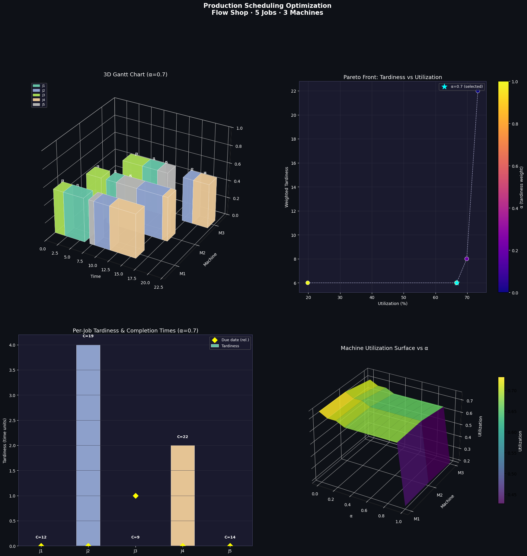
Figure saved.
Insights
Why J3 tends to be tardy — J3 has the tightest due date ($d=10$) but is not the shortest job; its high weight ($w=3$) makes the solver eager to schedule it early, yet upstream machines may already be occupied.
Utilization plateau — beyond $\alpha \approx 0.5$, pushing further toward pure tardiness minimization yields almost no additional tardiness reduction, but utilization can drop noticeably. This plateau, visible in Panel B, is the natural operating point for most factories.
Machine M2 bottleneck — the utilization surface (Panel D) shows M2 consistently at high utilization regardless of $\alpha$, identifying it as the system bottleneck. Investing in additional M2 capacity would shift the entire Pareto front favorably.
Scalability note — the position-indexed ILP has $O(J^2)$ binary variables and $O(J^2 \cdot M)$ disjunctive constraints. For $J \leq 12$ CBC solves in seconds. Beyond that, metaheuristics (simulated annealing, genetic algorithms) or branch-and-price methods become necessary.