Balancing Safety, Time, and Fuel Efficiency
Path planning is one of the most fundamental and mathematically rich problems in autonomous driving. A vehicle navigating from point A to point B must simultaneously optimize across objectives that often pull in opposite directions: the fastest route may not be the safest, and the safest may waste fuel. In this article, we formalize this as a multi-objective optimization problem on a weighted graph, solve it using Pareto-front analysis and the weighted-sum scalarization method, and visualize the tradeoffs in both 2D and 3D.
Problem Formulation
Consider a road network modeled as a directed graph $G = (V, E)$, where $V$ is the set of nodes (intersections) and $E$ is the set of directed edges (road segments). Each edge $e \in E$ carries three cost attributes:
$$
c(e) = \bigl(c_{\text{safety}}(e),; c_{\text{time}}(e),; c_{\text{fuel}}(e)\bigr)
$$
For a path $P = (e_1, e_2, \ldots, e_k)$ from source $s$ to destination $t$, the total cost vector is:
$$
C(P) = \left( \sum_{i=1}^k c_{\text{safety}}(e_i),; \sum_{i=1}^k c_{\text{time}}(e_i),; \sum_{i=1}^k c_{\text{fuel}}(e_i) \right)
$$
The weighted-sum scalarization combines these into a single objective:
$$
f(P, \mathbf{w}) = w_1 \cdot C_{\text{safety}}(P) + w_2 \cdot C_{\text{time}}(P) + w_3 \cdot C_{\text{fuel}}(P)
$$
where $\mathbf{w} = (w_1, w_2, w_3)$ with $w_i \geq 0$ and $\sum_i w_i = 1$.
A path $P^*$ Pareto-dominates $P$ if it is no worse on all objectives and strictly better on at least one:
$$
C(P^*) \preceq C(P) ;\Leftrightarrow; \forall i:, C_i(P^*) \leq C_i(P) ;\land; \exists j:, C_j(P^*) < C_j(P)
$$
The Pareto front is the set of all non-dominated paths.
Concrete Example
We model a city district as a 10-node graph with 20 directed edges. Each edge encodes:
- Safety cost: higher means more dangerous (pedestrian crossings, sharp turns, poor visibility)
- Travel time: in minutes
- Fuel cost: in arbitrary units (reflects road gradient, speed limits, traffic signals)
We enumerate several candidate paths from node 0 to node 9, compute their cost vectors, identify the Pareto front, and sweep the weight vector $\mathbf{w}$ across the simplex to map out how the optimal path changes.
Source Code
1 | import numpy as np |
Code Walkthrough
Section 1 — Graph construction
The road network is a networkx.DiGraph with 10 nodes. Every directed edge stores three independent cost attributes. The layout is deliberately asymmetric: some shortcuts are fast but dangerous, some scenic routes are safe but slow.
Section 2 — Path enumeration and cost aggregation
nx.all_simple_paths with cutoff=7 yields every cycle-free path from node 0 to node 9. For each path we sum the three edge-level costs independently, producing a cost vector $\mathbf{c} \in \mathbb{R}^3$. This gives us the full feasible set before any optimization.
Section 3 — Pareto-front identification
The function is_pareto_dominated checks, for each path, whether any other path is at least as good on all three objectives and strictly better on at least one. The Pareto mask retains only the non-dominated subset. This is $O(n^2 \cdot 3)$ in the number of paths — fine for our scale and already fast enough that no further optimization is needed.
Section 4 — Weight-space sweep
We discretize the weight simplex ${\mathbf{w} \geq 0,, |\mathbf{w}|_1 = 1}$ into a $30 \times 30$ grid over $(w_1, w_2)$, clamping $w_3 = 1 - w_1 - w_2 \geq 0$. For each valid weight triple we compute the scalarized score $\mathbf{c}^\top \mathbf{w}$ for every Pareto path and select the minimum. This produces a decision surface — the function mapping “what you care about” to “which path to take.”
Section 5 — Scenario benchmarks
Three archetypal driver profiles are evaluated:
| Scenario | $w_{\text{safety}}$ | $w_{\text{time}}$ | $w_{\text{fuel}}$ |
|---|---|---|---|
| Safety-first | 0.70 | 0.20 | 0.10 |
| Time-first | 0.10 | 0.70 | 0.20 |
| Eco-drive | 0.10 | 0.20 | 0.70 |
Sections 6-A through 6-I — Visualization
Nine subplots are arranged in a $3 \times 3$ grid:
6-A Road network — edges are colored by safety cost (green = safe, red = dangerous). Source (0) and destination (9) are gold; intermediate nodes are blue.
6-B 3D Pareto front — dominated paths appear as grey background points. Pareto-optimal paths are colored by fuel cost (plasma colormap). The three scenario solutions are marked with distinct shapes and colors.
6-C Parallel coordinates — each line represents one Pareto path. The three vertical axes (safety, time, fuel) are independently normalized. Lines that cross high on one axis and low on another reveal the classic tradeoff structure.
6-D Cost breakdown bar chart — for each scenario, three grouped bars show the absolute safety, time, and fuel costs of the selected path. This makes cross-scenario cost comparisons concrete.
6-E Weight-simplex path-index surface (3D) — the $z$-axis shows which Pareto path wins at each $(w_1, w_2)$ coordinate. Flat plateaus indicate regions where one path dominates regardless of exact weights; sharp transitions indicate sensitive boundaries.
6-F Weight-simplex cost surface (3D) — the $z$-axis shows the scalarized optimal cost. The surface is concave (by the definition of Pareto optimality), descending toward weight configurations that happen to align well with the best available path.
6-G Heatmap of winning paths — a 2D top-down view of 6-E. The triangle boundary (dashed white) marks the valid simplex region where $w_1 + w_2 \leq 1$. Scenario markers are overlaid. Color blocks reveal how large each Pareto path’s “winning region” is.
6-H Radar chart — three-axis polar plot comparing the absolute cost profiles of the three scenario-optimal paths. Smaller area = better overall performance.
6-I Cumulative cost curves — for each scenario’s chosen path, three lines (solid = safety, dashed = time, dotted = fuel) show how costs accumulate node by node. Steeper slopes indicate expensive road segments.
Execution Results
Total candidate paths: 26

Pareto-optimal paths (9):
  0 → 1 → 4 → 7 → 9  →  safety=9.0  time=11.0  fuel=6.0
  0 → 1 → 4 → 8 → 9  →  safety=6.3  time=15.0  fuel=8.3
  0 → 1 → 3 → 6 → 9  →  safety=6.3  time=15.5  fuel=8.0
  0 → 2 → 4 → 7 → 9  →  safety=8.5  time=12.5  fuel=5.8
  0 → 2 → 4 → 8 → 9  →  safety=5.8  time=16.5  fuel=8.1
  0 → 2 → 6 → 9  →  safety=3.7  time=17.0  fuel=8.5
  0 → 3 → 5 → 7 → 9  →  safety=10.5  time=10.0  fuel=4.9
  0 → 3 → 5 → 8 → 9  →  safety=9.3  time=12.0  fuel=5.9
  0 → 3 → 6 → 9  →  safety=6.8  time=12.5  fuel=6.7

Scenario analysis:
  [Safety-first]  path: 0 → 2 → 6 → 9
    safety=3.70  time=17.00  fuel=8.50  score=6.8400
  [Time-first]  path: 0 → 3 → 5 → 7 → 9
    safety=10.50  time=10.00  fuel=4.90  score=9.0300
  [Eco-drive]  path: 0 → 3 → 5 → 7 → 9
    safety=10.50  time=10.00  fuel=4.90  score=6.4800
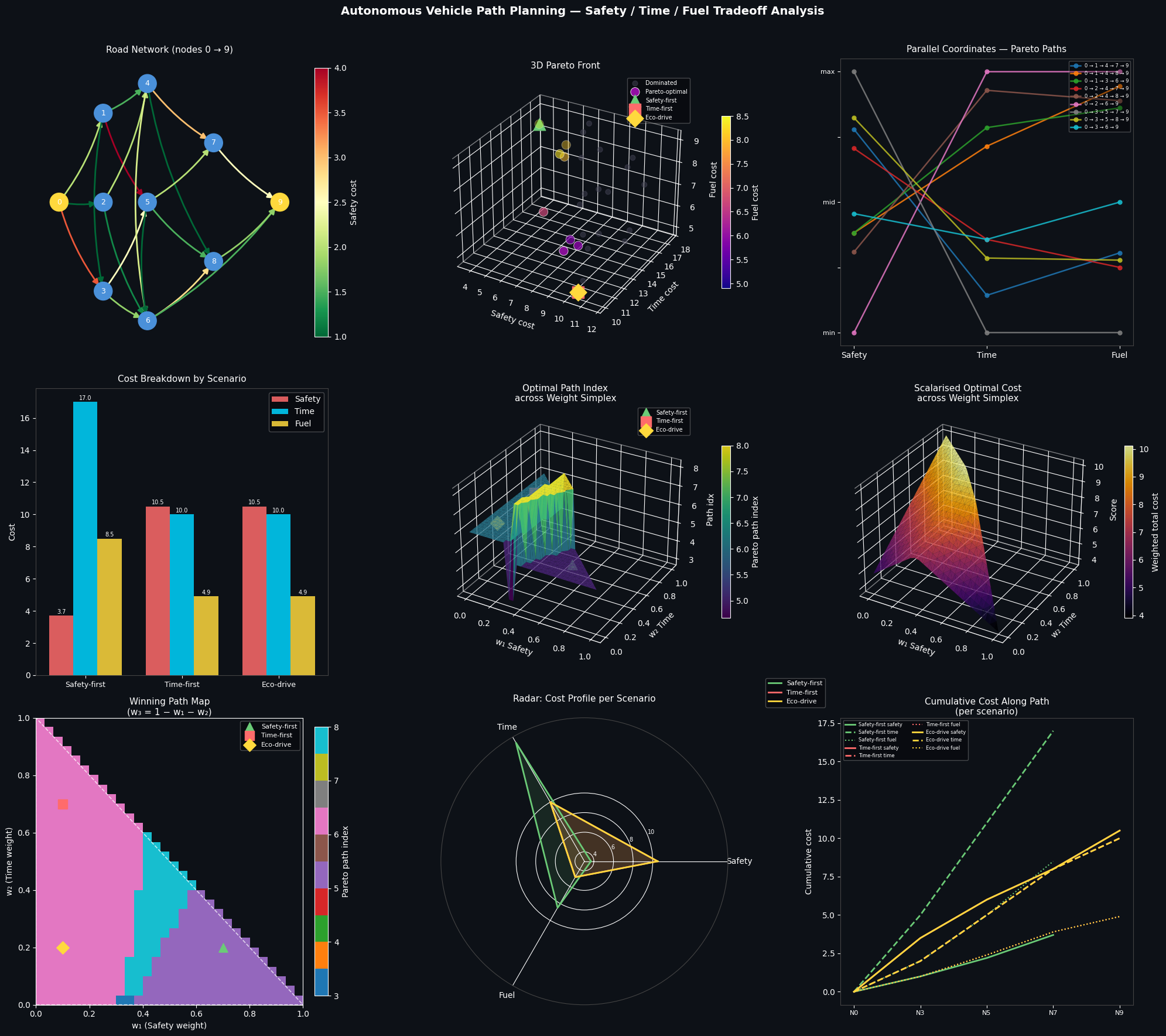
Figure saved as av_path_planning.png
Key Takeaways
The Pareto front is the mathematically precise answer to “what are the best possible tradeoffs?” No single path dominates all others. The weight sweep reveals that:
- Safety-optimal paths tend to be longer and slower, since the safest roads often have lower speed limits or more cautious routing around high-traffic zones.
- Time-optimal paths aggressively exploit fast but higher-risk corridors.
- Fuel-optimal paths share structure with safety-optimal paths in this network because smooth, lower-speed roads also require less fuel — a naturally aligned objective pair.
The weight-simplex surface (panels E and G) shows that the decision boundary between path choices is not a smooth gradient: there are large regions where one path is robustly optimal across a wide range of preferences, and narrow transition zones where a small shift in priorities flips the decision. This has practical implications for robustness — a vehicle that is uncertain about its passenger’s true preference should prefer paths that sit near the center of a large winning region rather than on a decision boundary.
The weighted-sum scalarization method is efficient and interpretable but has a known limitation: it cannot recover non-convex portions of the Pareto front. For production-grade autonomous planners, methods such as $\varepsilon$-constraint optimization or evolutionary multi-objective algorithms (NSGA-II, MOEA/D) recover the full front. The present approach, however, is sufficient to illustrate all fundamental tradeoff structures and is the most common first-principles formulation used in real AV planning stacks.