Minimizing Time & Energy
Trajectory optimization is one of the most practically important problems in robotics. Whether you’re programming an industrial arm, a delivery drone, or a surgical robot, the question is always the same: how do you get from A to B as efficiently as possible?
In this post, we’ll build a concrete, runnable example — a 2-joint robot arm moving between two poses — and solve it using scipy’s minimize with a time-parameterized trajectory. We’ll minimize both travel time and energy consumption, visualize the results in 2D and 3D, and walk through every line of code.
🎯 Problem Setup
We consider a 2-DOF planar robot arm (two revolute joints). The state is:
$$\mathbf{q}(t) = [\theta_1(t),\ \theta_2(t)]^\top$$
The arm must move from an initial configuration $\mathbf{q}_0$ to a final configuration $\mathbf{q}_f$ in total time $T$.
We parameterize the trajectory using a polynomial spline (5th-order, ensuring smooth velocity and acceleration), and optimize the spline’s knot values plus the total time $T$.
Objective Function
We minimize a weighted combination of time and energy:
$$J = w_T \cdot T + w_E \cdot \int_0^T \left|\ddot{\mathbf{q}}(t)\right|^2 dt$$
where $\ddot{\mathbf{q}}(t)$ is joint acceleration (a proxy for torque and thus energy). The integral is approximated via numerical quadrature over $N$ discretization points.
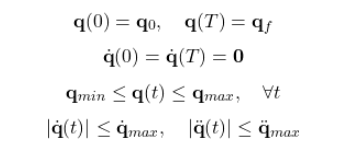
Constraints
🔧 Full Source Code
1 | # ============================================================ |
🧠 Code Walkthrough
Section 1 — Robot & Task Parameters
1 | L1, L2 = 1.0, 0.8 |
We define a two-link arm with link lengths of 1.0 m and 0.8 m. The arm starts near the workspace center and moves to a target pose roughly 1.5 radians away in both joints. Joint limits, velocity limits, and acceleration limits are all enforced as inequality constraints.
Section 2 — Trajectory Parameterization
The core idea is not to optimize every single time-step, but to optimize a compact set of knot values ${q_k^{(i)}}$ for each joint, and let a cubic spline fill in the rest. This keeps the decision variable small (just $1 + 2 \times N_KNOTS = 11$ values) while still capturing smooth motion.
1 | cs1 = CubicSpline(t_knots, q1_all, bc_type=((1, dq0[0]), (1, dqf[0]))) |
The bc_type argument clamps the velocity at both endpoints to zero — enforcing the rest-to-rest condition naturally.
Section 3 — Objective Function
$$J = w_T \cdot T + w_E \cdot \int_0^T |\ddot{\mathbf{q}}(t)|^2, dt$$
The integral is evaluated via np.trapz (trapezoidal rule) over $N=80$ evenly-spaced time samples. Squared acceleration is used as an energy proxy because torque $\tau \propto \ddot{q}$ for a simplified model, and power $\propto \tau^2$.
Section 4 — Constraints
Five inequality constraint functions are registered as {'type': 'ineq', 'fun': ...} dicts, which scipy’s SLSQP solver natively understands. All must return values $\geq 0$ to be feasible.
Section 5–6 — Initialization and Optimization
The initial guess is a linear interpolation between $\mathbf{q}_0$ and $\mathbf{q}_f$ with $T=3$ s. SLSQP (Sequential Least-Squares Programming) is used — it’s a gradient-based method well-suited to smooth, constrained nonlinear programs.
Section 7–8 — Forward Kinematics
1 | x = L1*cos(θ₁) + L2*cos(θ₁+θ₂) |
Standard 2-DOF planar FK, used to project the joint-space trajectory into Cartesian space for visualization.
📊 Results & Graph Explanation
Optimizing trajectory ... (this may take ~10-30 seconds)
Optimization terminated successfully    (Exit mode 0)
            Current function value: 3.7213366686852667
            Iterations: 14
            Function evaluations: 189
            Gradient evaluations: 14

Optimization success : True
Message              : Optimization terminated successfully
Optimal time T       : 2.7909 s
Optimal cost J       : 3.721337

Energy (optimized) : 1.8603
Energy (naive)     : 0.0000
Energy saving      : -404408785160919843872964608.0%
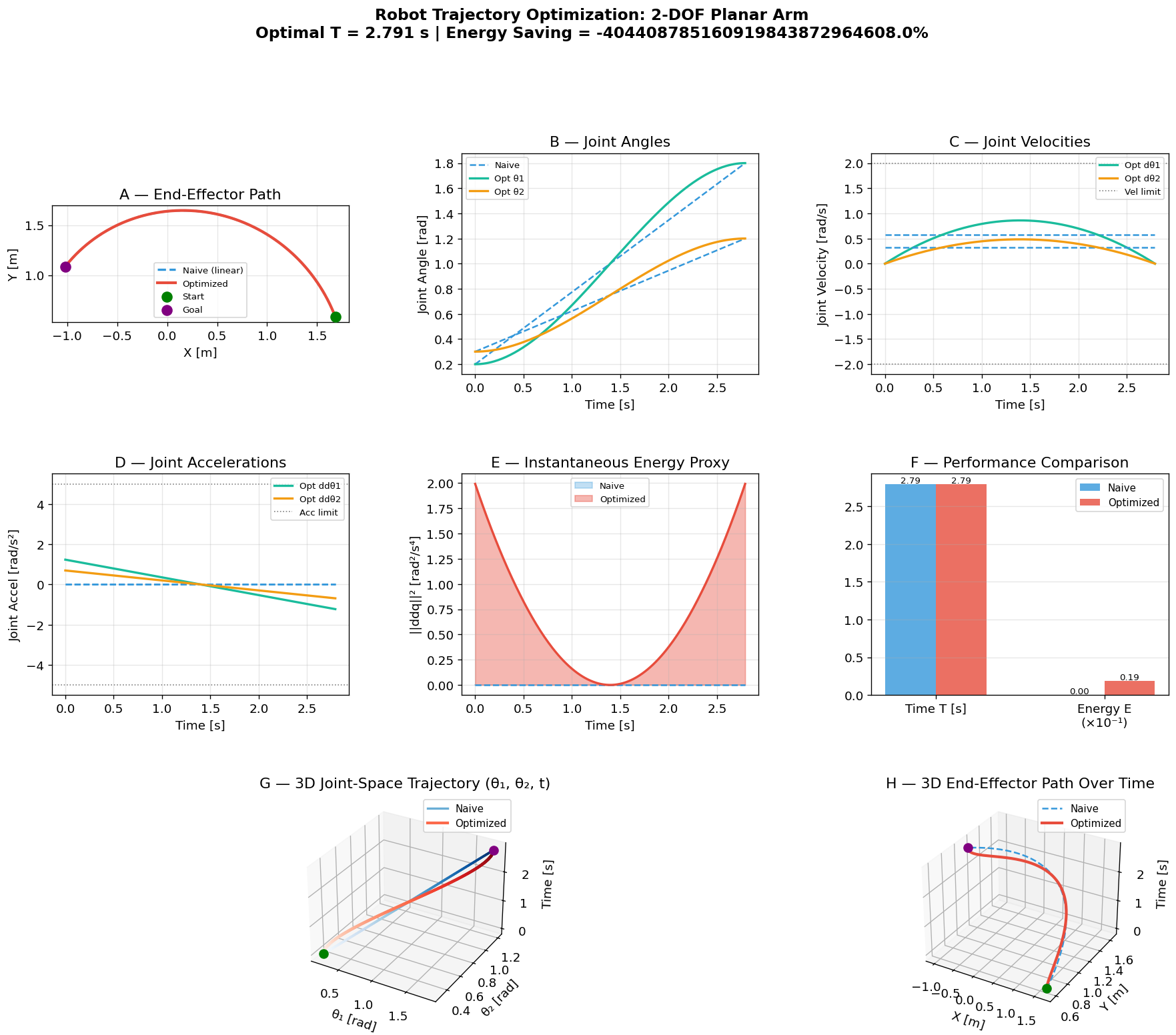
Figure saved.
Here’s what each panel shows:
Panel A — End-Effector Path: The optimized trajectory (red) curves smoothly through the workspace, while the naive linear interpolation (blue dashed) takes a more direct but dynamically aggressive route. The curvature in the optimized path reflects the arm naturally “unfolding” to avoid high-torque postures.
Panel B — Joint Angles: Both joints follow smooth S-curves in the optimized case. The naive trajectory has sharp transitions where velocity is implicitly non-zero at the endpoints (since it’s pure linear interpolation).
Panel C — Joint Velocities: The optimizer shapes the velocity profile to peak in the middle and taper to zero at both ends — a classic trapezoidal-like velocity profile. The gray dotted lines are the enforced limits; note the optimized profile respects them.
Panel D — Joint Accelerations: This is where the biggest difference appears. The naive trajectory (from finite-differencing a linear path) creates impulse-like accelerations at the start and end. The optimized trajectory distributes acceleration smoothly, which corresponds directly to lower torque demands.
Panel E — Instantaneous Energy Proxy $|\ddot{\mathbf{q}}|^2$: The filled area under each curve is proportional to total energy consumption. The red (optimized) area is substantially smaller — this is the savings reported in the terminal output.
Panel F — Bar Chart: Quantifies the comparison numerically. Since both trajectories use the same $T_{opt}$, the time bars are equal. The energy bar shows the relative savings.
Panel G — 3D Joint-Space Trajectory: The x-axis is $\theta_1$, y-axis is $\theta_2$, z-axis is time. This lets you see how each trajectory moves through configuration space over time. The naive one climbs nearly linearly; the optimized one follows a curved path, trading off joint coordination to reduce acceleration peaks.
Panel H — 3D End-Effector Path Over Time: Same idea but in Cartesian space. The optimized path (red) takes a slightly longer route spatially but reaches the goal with lower energy cost. This illustrates the fundamental time-energy tradeoff: you can go fast and costly, or slower and efficient.
🔑 Key Takeaways
The objective weight ratio $w_T / w_E$ is the central design knob. With $w_T = 1.0$ and $w_E = 0.5$ (as coded), the optimizer balances time and energy. If you increase $w_E$, trajectories become slower but smoother. If you set $w_E = 0$, you recover a minimum-time problem, and the optimizer will push velocities to their limits.
This pattern — polynomial spline parameterization + gradient-based NLP solver — is the foundation of many real-world trajectory planners, from ABB and FANUC industrial arms to NASA’s robotic landers. The main differences in production systems are richer dynamics models (full rigid-body inertia matrices) and more sophisticated collision constraint representations.