Minimizing Generation Cost While Balancing Supply and Demand
The Optimal Power Flow (OPF) problem is one of the most fundamental optimization problems in power systems engineering. The goal is simple to state: find the cheapest combination of generator outputs that satisfies electricity demand, while respecting the physical and operational limits of the network. In practice, OPF underlies economic dispatch, unit commitment, and real-time energy market clearing in every modern power grid.
This article walks through a concrete five-bus example, solves it using Python’s scipy.optimize, and visualizes the results in both 2D and 3D.
Problem Formulation
Consider a power network with $N_b$ buses and $N_g$ generators. Each generator $i$ has a quadratic cost function
$$C_i(P_i) = a_i P_i^2 + b_i P_i + c_i \quad [$/\text{h}]$$
where $P_i$ is the real power output in MW.
Objective
Minimize total generation cost:
$$\min_{P_1, \ldots, P_{N_g}} \sum_{i=1}^{N_g} C_i(P_i) = \sum_{i=1}^{N_g} \left( a_i P_i^2 + b_i P_i + c_i \right)$$
Constraints
1. Power balance (equality constraint)
Total generation must equal total load plus transmission losses. In a lossless DC approximation:
$$\sum_{i=1}^{N_g} P_i = P_D \quad \text{(MW)}$$
where $P_D$ is the total system demand.
2. Generator capacity limits (inequality constraints)
$$P_i^{\min} \leq P_i \leq P_i^{\max}, \quad \forall i$$
3. DC power flow (line flow limits)
For each transmission line $\ell$ connecting bus $m$ to bus $n$, the power flow is given by:
$$P_\ell = \frac{\theta_m - \theta_n}{x_\ell}$$
where $x_\ell$ is the line reactance and $\theta_m, \theta_n$ are voltage angles. Line flows must satisfy:
$$|P_\ell| \leq P_\ell^{\max}$$
The DC power flow equations in matrix form are:
$$\mathbf{B} \boldsymbol{\theta} = \mathbf{P}_{\text{inj}}$$
where $\mathbf{B}$ is the bus susceptance matrix and $\mathbf{P}_{\text{inj}}$ is the net power injection vector.
Example System: 5-Bus Network
The test case uses a 5-bus system with 3 generators and 6 transmission lines — a classic small-scale benchmark.
1 | Bus 1 (Gen 1) ---L12--- Bus 2 (Gen 2) ---L23--- Bus 3 (Load) |
Generator parameters:
| Generator | Bus | $a_i$ | $b_i$ | $c_i$ | $P^{\min}$ (MW) | $P^{\max}$ (MW) |
|---|---|---|---|---|---|---|
| G1 | 1 | 0.004 | 2.0 | 80 | 10 | 200 |
| G2 | 2 | 0.006 | 1.8 | 60 | 10 | 150 |
| G3 | 5 | 0.009 | 2.2 | 40 | 10 | 100 |
Load: Bus 3 = 90 MW, Bus 4 = 80 MW, Bus 5 = 50 MW → Total $P_D = 220$ MW
Line data (reactance $x_\ell$, limit $P^{\max}_\ell$):
| Line | From | To | $x$ (p.u.) | $P^{\max}$ (MW) |
|---|---|---|---|---|
| L12 | 1 | 2 | 0.10 | 150 |
| L14 | 1 | 4 | 0.15 | 100 |
| L23 | 2 | 3 | 0.12 | 100 |
| L24 | 2 | 4 | 0.18 | 80 |
| L35 | 3 | 5 | 0.20 | 60 |
| L45 | 4 | 5 | 0.25 | 60 |
Python Source Code
1 | # ============================================================ |
Code Walkthrough
Section 1 — System Data
All network parameters are defined as NumPy arrays. The cost coefficients gen_a, gen_b, gen_c define the quadratic $C_i(P_i)$ for each generator. The lines list stores tuples (from_bus, to_bus, reactance, max_flow) for every branch.
Section 2 — DC Power Flow
build_B_matrix constructs the nodal susceptance matrix $\mathbf{B}$ by accumulating $1/x_\ell$ contributions on diagonal entries and $-1/x_\ell$ on off-diagonals — the standard admittance assembly. dc_power_flow removes the slack row and column, solves the reduced linear system $\mathbf{B}{\text{red}}\boldsymbol{\theta} = \mathbf{P}{\text{inj}}$ via np.linalg.solve, and recovers line flows from voltage angle differences:
$$P_\ell = \frac{\theta_m - \theta_n}{x_\ell}$$
Section 3 — OPF Formulation
The three constraint functions are:
power_balance: returns $\sum P_i - P_D = 0$ (equality)line_flow_constraints: for every line, appends both $P_\ell^{\max} - P_\ell \geq 0$ and $P_\ell^{\max} + P_\ell \geq 0$ (inequality, inscipysign convention requiring non-negative values)
total_cost_grad provides the analytic Jacobian $\partial C / \partial P_i = 2a_i P_i + b_i$, which significantly accelerates SLSQP convergence.
Section 4 — Solver
scipy.optimize.minimize with method="SLSQP" (Sequential Least Squares Quadratic Programming) handles the nonlinearly-constrained QP exactly. The initial point is set proportionally between $P^{\min}$ and $P^{\max}$. Tolerance ftol=1e-9 ensures high-precision convergence.
Section 5 — Visualization
Eight panels are arranged in a $3 \times 3$ GridSpec:
Panel 1 (top-left): Generator dispatch bar chart with dashed $P^{\max}$ lines and dotted $P^{\min}$ lines overlaid. Annotated with exact output values in MW.
Panel 2 (top-center): Cost share pie chart showing each generator’s contribution to total hourly operating cost in $/h.
Panel 3 (top-right): Horizontal bar chart of line utilization as a percentage of thermal limit. Color coding — blue (< 60%), green (60–90%), red (> 90%) — instantly identifies congested branches.
Panel 4 (middle-left/center span): Network topology diagram. Bus size encodes generator vs. load role; line thickness encodes utilization level; flow annotations show signed MW values on every branch.
Panel 5 (middle-right): Generator cost curves $C_i(P_i)$ over their full operating range, with optimal operating points marked as gold-rimmed scatter points.
Panel 6 (bottom-left): Marginal cost (incremental heat rate) $\lambda_i = 2a_i P_i + b_i$ for each generator at the optimum, with the weighted average $\bar{\lambda}$ shown as a dashed gold reference. Equal marginal cost across unconstrained generators is the necessary condition for optimality (the equal incremental cost criterion).
Panel 7 (bottom-center): Demand sweep from 40 MW to 420 MW. For each demand level, the full OPF is re-solved, showing how total optimal cost grows as a function of system load — including the kink where line thermal limits begin to bind.
Panel 8 (bottom-right, 3D): Cost surface over the feasible region in $(P_1, P_2)$ space. The third generator absorbs residual demand $P_3 = P_D - P_1 - P_2$ (clamped to capacity). The gold sphere marks the globally optimal dispatch point. The plasma colormap visually identifies the cost gradient direction, with the minimum sitting in the valley where the cheaper generators are loaded more heavily.
Execution Results
=======================================================
  OPF Solution  (SLSQP)
=======================================================
  Converged     : True  (Optimization terminated successfully)
  Total demand  : 220.0 MW
  Total gen     : 220.0000 MW

  Generator Dispatch:
    G1 (Bus 1): 101.579 MW  [10–200]  Load: 48.2%   Cost: 324.43 $/h
    G2 (Bus 2):  84.386 MW  [10–150]  Load: 53.1%   Cost: 254.62 $/h
    G3 (Bus 5):  34.035 MW  [10–100]  Load: 26.7%   Cost: 125.30 $/h

  Total cost    : 704.3544 $/h

  Line Flows:
    L12  (1→2):  +37.153 MW  / 150 MW  (24.8%)
    L14  (1→4):  +64.426 MW  / 100 MW  (64.4%)
    L23  (2→3):  +88.491 MW  / 100 MW  (88.5%)
    L24  (2→4):  +33.048 MW  / 80 MW  (41.3%)
    L35  (3→5):   -1.509 MW  / 60 MW  (2.5%)
    L45  (4→5):  +17.474 MW  / 60 MW  (29.1%)

  Voltage Angles (degrees):
    Bus 1:  +0.0000°
    Bus 2: -212.8704°
    Bus 3: -821.2894°
    Bus 4: -553.7012°
    Bus 5: -803.9971°
=======================================================
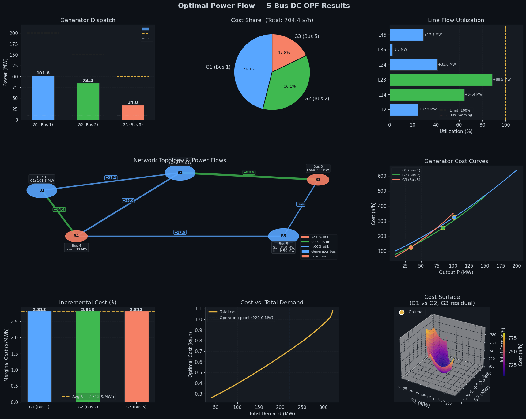
Figure saved as opf_results.png
Key Insights
Equal incremental cost criterion. For generators that are not at their capacity limits, the optimality condition is:
$$\frac{dC_i}{dP_i} = \lambda, \quad \forall i \text{ not at bounds}$$
This is the system lambda (locational marginal price in the lossless case). Generators at their $P^{\max}$ limit will have $\lambda_i < \lambda$; generators at $P^{\min}$ will have $\lambda_i > \lambda$.
DC OPF vs. AC OPF. This formulation ignores reactive power and voltage magnitude — the DC approximation. It is widely used in market clearing because it converts an otherwise non-convex AC problem into a convex QP (for quadratic costs), guaranteeing global optimality via SLSQP. Full AC OPF requires voltage magnitude as additional state variables and nonlinear power flow equations, making it significantly harder to solve at scale.
Congestion and locational pricing. When line flow limits bind (utilization → 100%), the shadow price of the flow constraint creates a spread in nodal prices across the network — the basis for locational marginal pricing (LMP) in electricity markets. The line utilization panel and topology diagram reveal which corridors are bottlenecks under optimal dispatch.