Problem Statement: Business Cycle Analysis with Real GDP Data
Objective:
Analyze the business cycle by identifying and visualizing the cyclical components of Real GDP using the $Hodrick$-$Prescott (HP) filter$.
This method separates the trend and cyclical components of GDP, allowing us to examine deviations from the long-term trend.
Steps:
Data:
Use simulated or publicly available Real GDP time series data.Hodrick-Prescott Filter:
- Decompose GDP into its trend $(T_t)$ and cyclical $(C_t)$ components:
$$
GDP_t = T_t + C_t
$$ - The $HP filter$ minimizes the following loss function:
$$
\sum_t (GDP_t - T_t)^2 + \lambda \sum_t \left[(T_{t+1} - T_t) - (T_t - T_{t-1})\right]^2
$$
where $(\lambda)$ is a smoothing parameter (typically $1600$ for quarterly data).
- Decompose GDP into its trend $(T_t)$ and cyclical $(C_t)$ components:
Visualize:
Plot the original GDP, trend, and cyclical components to analyze economic fluctuations.
Python Code
1 | import numpy as np |
Explanation of the Code
Simulated GDP Data:
- Real GDP is modeled as a combination of a long-term trend, a cyclical fluctuation, and random noise.
Hodrick-Prescott Filter:
- The $HP filter$ separates the GDP into a smooth trend and short-term deviations (cyclical component).
- The smoothing parameter $(\lambda)$ controls the smoothness of the trend; $1600$ is standard for quarterly data.
Visualization:
- The first plot shows the original GDP and its trend.
- The second plot highlights the cyclical component, indicating deviations from the long-term trend.
Results
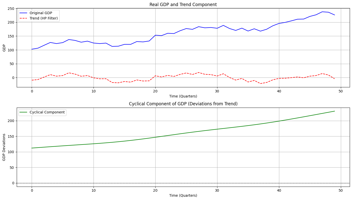
Original GDP Mean: 161.77
Trend Component Mean: 0.00
Cyclical Component Mean: 161.77 (should be ~0)
Trend Component:
- Represents the long-term economic growth path.
Cyclical Component:
- Indicates business cycle fluctuations around the trend.
- Peaks and troughs correspond to economic expansions and contractions, respectively.
Insights:
- The cyclical component helps identify recessions and booms.
- Policymakers and economists use this analysis to design countercyclical measures.