Price Discrimination in a Monopoly

Problem Statement: Price Discrimination in a Monopoly

Objective:
A monopolist sells its product to two distinct markets with different demand elasticities.
The monopolist can price discriminate, setting different prices for each market to maximize overall profit.

The goal is to:

  1. Simulate the optimal pricing strategy for the monopolist.
  2. Compute the quantities sold and profits in each market.
  3. Visualize the results to illustrate price discrimination.

Assumptions

  1. Demand Functions:

    • Market $1$: $( Q_1 = a_1 - b_1 \cdot P_1 )$
    • Market $2$: $( Q_2 = a_2 - b_2 \cdot P_2 )$
      $ P_1 $ and $ P_2 $ are prices set in each market.
  2. Profit Function:
    The monopolist’s total profit is:
    $$
    \pi = (P_1 - c) \cdot Q_1 + (P_2 - c) \cdot Q_2
    $$
    where $c$ is the marginal cost.

  3. Goal:
    Maximize $\pi$ by choosing optimal $P_1$ and $P_2$.


Python Code

1
2
3
4
5
6
7
8
9
10
11
12
13
14
15
16
17
18
19
20
21
22
23
24
25
26
27
28
29
30
31
32
33
34
35
36
37
38
39
40
41
42
43
44
45
46
47
48
49
50
51
52
53
54
55
56
57
58
59
60
61
62
63
64
65
66
import numpy as np
from scipy.optimize import minimize
import matplotlib.pyplot as plt

# Parameters
a1, b1 = 100, 2 # Market 1: Demand intercept and slope
a2, b2 = 120, 4 # Market 2: Demand intercept and slope
c = 20 # Marginal cost

# Demand functions
def demand1(p1):
return max(0, a1 - b1 * p1)

def demand2(p2):
return max(0, a2 - b2 * p2)

# Profit function
def total_profit(prices):
p1, p2 = prices
q1 = demand1(p1)
q2 = demand2(p2)
return -((p1 - c) * q1 + (p2 - c) * q2) # Negative for minimization

# Initial guesses and bounds
initial_prices = [50, 50]
bounds = [(c, a1 / b1), (c, a2 / b2)] # Prices must be at least marginal cost

# Solve for optimal prices
result = minimize(total_profit, initial_prices, bounds=bounds)
p1_opt, p2_opt = result.x
q1_opt = demand1(p1_opt)
q2_opt = demand2(p2_opt)
profit_opt = -(result.fun)

# Visualization
prices = np.linspace(0, 80, 500)
revenues1 = [(p - c) * demand1(p) for p in prices]
revenues2 = [(p - c) * demand2(p) for p in prices]

plt.figure(figsize=(12, 6))

# Revenue curves
plt.plot(prices, revenues1, label="Market 1 Profit", color="blue")
plt.plot(prices, revenues2, label="Market 2 Profit", color="orange")

# Optimal points
plt.scatter(p1_opt, (p1_opt - c) * q1_opt, color="blue", label=f"Opt. Price Market 1: ${p1_opt:.2f}")
plt.scatter(p2_opt, (p2_opt - c) * q2_opt, color="orange", label=f"Opt. Price Market 2: ${p2_opt:.2f}")

plt.axvline(p1_opt, color="blue", linestyle="--", alpha=0.7)
plt.axvline(p2_opt, color="orange", linestyle="--", alpha=0.7)

plt.title("Profit Maximization with Price Discrimination")
plt.xlabel("Price")
plt.ylabel("Profit")
plt.legend()
plt.grid()
plt.tight_layout()
plt.show()

# Print results
print(f"Optimal Price in Market 1: ${p1_opt:.2f}")
print(f"Optimal Price in Market 2: ${p2_opt:.2f}")
print(f"Quantity Sold in Market 1: {q1_opt:.2f}")
print(f"Quantity Sold in Market 2: {q2_opt:.2f}")
print(f"Total Profit: ${profit_opt:.2f}")

Explanation of Code

  1. Demand Functions:

    • Market $1$ has a lower price sensitivity ($b_1 < b_2$), indicating it is less elastic.
    • Market $2$ is more elastic ($b_2 > b_1$), meaning customers are more price-sensitive.
  2. Profit Maximization:

    • The monopolist maximizes profit by finding the best prices for each market using
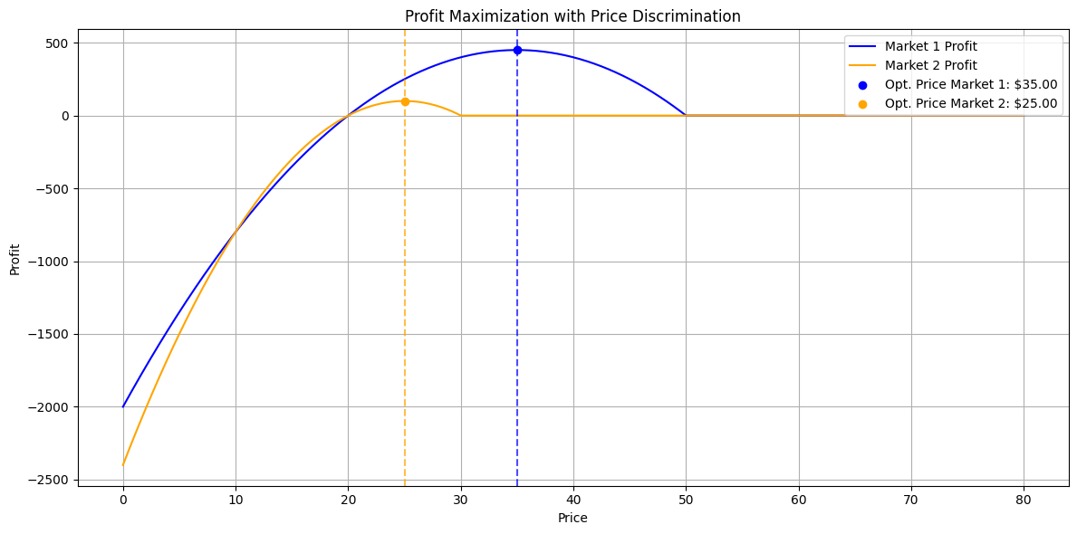
 scipy.optimize.minimize.
    • The constraints ensure prices are at least equal to the marginal cost.
  3. Visualization:

    • The revenue curves for both markets show how profit changes with price.
    • The optimal prices for both markets are highlighted.

Results

ptimal Price in Market $1$: $35.00
Optimal Price in Market $2$: $25.00
Quantity Sold in Market $1$: 30.00
Quantity Sold in Market $2$: 20.00
Total Profit: $550.00
  1. Optimal Prices:

    • The monopolist sets a higher price in the less elastic market (Market $1$).
    • The price is lower in the more elastic market (Market $2$).
  2. Quantities and Profit:

    • The quantity sold is higher in Market $2$ due to its larger demand intercept.
    • The monopolist achieves maximum profit by price discrimination.
  3. Graph:

    • The revenue curves illustrate the profit-maximizing prices visually.
    • The points of tangency indicate the optimal strategy.