Problem Statement: Optimal Taxation and the Laffer Curve
The Laffer Curve illustrates the relationship between tax rates and government revenue.
At very low tax rates, government revenue is minimal, and at very high tax rates, revenue also decreases because of reduced economic activity.
The goal is to:
- Simulate the Laffer Curve based on a theoretical economy.
- Identify the optimal tax rate that maximizes government revenue.
- Visualize the results.
Python Code
1 | import numpy as np |
Explanation of the Code
- Economic Model:
- The
government_revenuefunction calculates revenue as (Revenue=Tax Rate×Economic Activity). - Economic activity decreases quadratically with higher tax rates, representing reduced incentives for productivity at high taxation levels.
- The
- Simulation:
- Tax rates range from 0% to 100%.
- Government revenue is computed for each tax rate.
- Optimization:
- The optimal tax rate corresponds to the maximum government revenue, determined using
np.argmax.
- The optimal tax rate corresponds to the maximum government revenue, determined using
- Visualization:
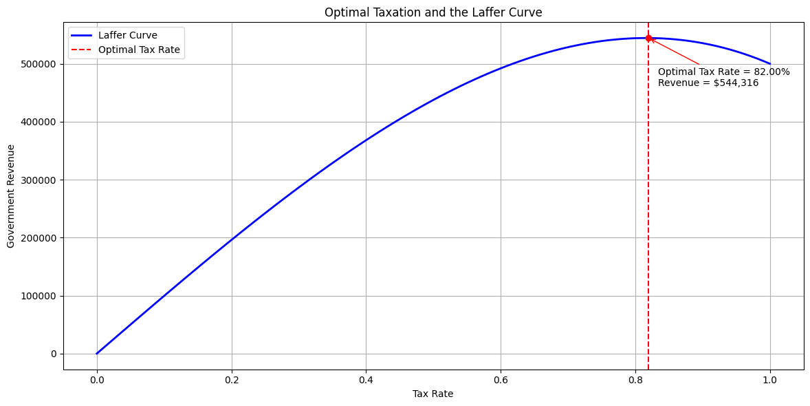
- The Laffer Curve shows the relationship between tax rates and revenue.
- The optimal tax rate is highlighted with a vertical line and annotated.
Results

- Laffer Curve:
- The curve rises as the tax rate increases initially but falls after a certain point due to reduced economic activity.
- Optimal Tax Rate:
- This is the tax rate where government revenue is maximized.
- The plot includes a clear marker and annotation for this point.