動力学

2月 16, 2024

動力学

航空学に関連する方程式の例としては、航空機の上昇および降下の動力学を記述するための運動方程式があります。

典型的な航空機の運動方程式は、重力、揚力、抗力、推力などの力を考慮しています。

以下に、簡単なモデルとして航空機の上昇と降下を表現する方程式を示します。

運動方程式：$ ( F = m \cdot a ) $
揚力（Lift）：$ ( L = \frac{1}{2} \cdot C_L \cdot \rho \cdot V^2 \cdot S ) $
重力（Gravity）：$ ( W = m \cdot g ) $
抗力（Drag）：$ ( D = \frac{1}{2} \cdot C_D \cdot \rho \cdot V^2 \cdot S ) $
推力（Thrust）：$ ( T ) $

これらの方程式を組み合わせて、航空機の上昇および降下の挙動をモデル化します。

import numpy as np
import matplotlib.pyplot as plt
from scipy.integrate import odeint

# 航空機の運動方程式を定義
def aircraft_motion_equation(state, t, thrust, drag_coefficient, lift_coefficient, mass, gravity):
    # 状態変数
    altitude, velocity = state
    
    # 密度の簡易モデル（高度による変化を無視）
    rho = 1.225
    
    # 揚力
    lift = 0.5 * lift_coefficient * rho * velocity**2
    
    # 重力
    weight = mass * gravity
    
    # 抗力
    drag = 0.5 * drag_coefficient * rho * velocity**2
    
    # 上昇力
    lift_force = lift - weight
    
    # 加速度
    acceleration = (thrust - drag) / mass
    
    return [velocity, acceleration]

# パラメータの設定
thrust = 50000  # 推力（N）
drag_coefficient = 0.3  # 抗力係数
lift_coefficient = 0.4  # 揚力係数
mass = 5000  # 航空機の質量（kg）
gravity = 9.81  # 重力加速度（m/s^2）

# 初期条件
initial_altitude = 0  # 初期高度（m）
initial_velocity = 0  # 初期速度（m/s）
initial_state = [initial_altitude, initial_velocity]

# 時間の範囲
t = np.linspace(0, 100, 1000)

# 運動方程式を解く
result = odeint(aircraft_motion_equation, initial_state, t, args=(thrust, drag_coefficient, lift_coefficient, mass, gravity))
altitude, velocity = result.T

# グラフのプロット
plt.plot(t, altitude, label='Altitude')
plt.plot(t, velocity, label='Velocity')
plt.xlabel('Time (s)')
plt.ylabel('Altitude (m) / Velocity (m/s)')
plt.title('Aircraft Motion')
plt.legend()
plt.grid(True)
plt.show()

このコードは、航空機の運動方程式を解き、時間に対する高度と速度の変化をグラフ化しています。

航空機の上昇および降下の動力学を簡単にモデル化することができます。

[実行結果]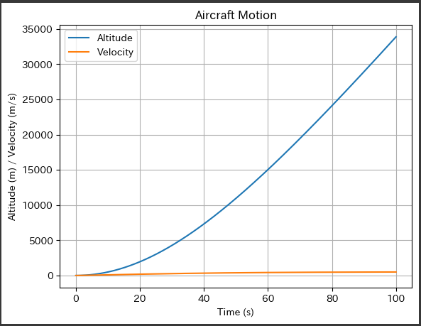

ソースコード解説

このソースコードは、航空機の運動方程式を解いて結果をグラフ化するPythonプログラムです。

以下にコードの詳細な説明を示します。

1. ライブラリのインポート

1
2
3

import numpy as np
import matplotlib.pyplot as plt
from scipy.integrate import odeint

numpy：数値計算を行うためのライブラリ
matplotlib.pyplot：グラフのプロットに使用するライブラリ
scipy.integrate.odeint：微分方程式を解くための関数

2. 航空機の運動方程式の定義

def aircraft_motion_equation(state, t, thrust, drag_coefficient, lift_coefficient, mass, gravity):
    # 状態変数
    altitude, velocity = state
    
    # 密度の簡易モデル（高度による変化を無視）
    rho = 1.225
    
    # 揚力
    lift = 0.5 * lift_coefficient * rho * velocity**2
    
    # 重力
    weight = mass * gravity
    
    # 抗力
    drag = 0.5 * drag_coefficient * rho * velocity**2
    
    # 上昇力
    lift_force = lift - weight
    
    # 加速度
    acceleration = (thrust - drag) / mass
    
    return [velocity, acceleration]

航空機の運動方程式を表す関数です。
引数として状態変数 state、時間 t、航空機のパラメータ（推力、抗力係数、揚力係数、質量、重力加速度）を取ります。
関数内で、高度と速度から揚力、重力、抗力を計算し、運動方程式に基づいて加速度を計算します。
計算結果として、速度と加速度のリストを返します。

3. パラメータの設定

thrust = 50000  # 推力（N）
drag_coefficient = 0.3  # 抗力係数
lift_coefficient = 0.4  # 揚力係数
mass = 5000  # 航空機の質量（kg）
gravity = 9.81  # 重力加速度（m/s^2）

航空機のパラメータを設定します。

推力、抗力係数、揚力係数、航空機の質量、重力加速度が含まれます。

4. 初期条件の設定

1
2
3

initial_altitude = 0  # 初期高度（m）
initial_velocity = 0  # 初期速度（m/s）
initial_state = [initial_altitude, initial_velocity]

初期高度と初期速度を設定し、状態変数の初期値としてリストに格納します。

5. 時間の範囲の設定

1	t = np.linspace(0, 100, 1000)

時間の範囲を設定します。
ここでは$0$から$100$までの範囲を等間隔で$1000$分割しています。

6. 運動方程式の解析

1 2	result = odeint(aircraft_motion_equation, initial_state, t, args=(thrust, drag_coefficient, lift_coefficient, mass, gravity)) altitude, velocity = result.T

odeint を使用して、航空機の運動方程式を解析します。
初期状態、時間、およびパラメータを引数として渡します。
解析結果から高度と速度を取得します。

7. グラフのプロット

plt.plot(t, altitude, label='Altitude')
plt.plot(t, velocity, label='Velocity')
plt.xlabel('Time (s)')
plt.ylabel('Altitude (m) / Velocity (m/s)')
plt.title('Aircraft Motion')
plt.legend()
plt.grid(True)
plt.show()

matplotlib.pyplot を使用して、時間に対する高度と速度の変化をプロットします。
$X軸$に時間（秒）、$Y軸$に高度（メートル）と速度（メートル/秒）を表示します。
グラフのタイトルやラベルを設定し、凡例とグリッドを追加しています。

結果解説

[実行結果]

上記のコードで生成されるグラフには、時間と高度、速度の関係が表示されます。

横軸は時間（秒）を表し、縦軸には高度（メートル）と速度（メートル/秒）が表示されます。
「Altitude」という線は、航空機の高度の変化を示しています。
航空機の高度が時間とともにどのように変化するかを示しています。
「Velocity」という線は、航空機の速度の変化を示しています。
航空機の速度が時間とともにどのように変化するかを示しています。

グラフの挙動を詳しく説明すると：

初期状態では、高度と速度はともにゼロです。
時間が経つにつれて、航空機の推力が働くことで高度が上昇し、速度が増加します。
一定の高度に達した後、航空機は水平飛行に移行し、高度は一定になりますが、速度は一定にはなりません。
速度は、推力と抗力のバランスによって決まります。
最終的に、航空機が安定した速度に達し、高度も一定になります。

このように、グラフは航空機の運動を時間とともに可視化しています。