ソーシャルメディア感情分析 scikit-learn

ソーシャルメディア感情分析

ソーシャルメディア感情分析の例題として、Twitterのツイートデータを使用して、テキストデータから感情（ポジティブ、ネガティブ、またはニュートラル）を予測する方法を示します。

感情分析には、自然言語処理の手法と機械学習アルゴリズムを組み合わせます。

まず、必要なライブラリをインポートします。

import numpy as np
import pandas as pd
import matplotlib.pyplot as plt
import seaborn as sns
import re
import nltk
from nltk.corpus import stopwords
from sklearn.feature_extraction.text import CountVectorizer
from sklearn.model_selection import train_test_split
from sklearn.naive_bayes import MultinomialNB
from sklearn.metrics import accuracy_score, confusion_matrix, classification_report

次に、Twitterの感情分析用のサンプルデータを用意します。

data = {
    'text': [
        "I love this product, it's amazing!",
        "This movie was terrible, never watching it again!",
        "Neutral tweet about some topic.",
        "The weather is beautiful today.",
        "Had a great time at the beach with friends!",
        "Feeling tired after a long day at work.",
        "Excited for the upcoming vacation!",
        "Disappointed with the customer service.",
        "Trying out a new recipe for dinner tonight.",
        "Can't wait to see my favorite band in concert!",
        "Feeling happy and grateful for all the love and support.",
        "Feeling overwhelmed with deadlines and tasks.",
        "Just finished reading a fantastic book!",
        "Feeling bored, looking for something fun to do.",
        "Feeling anxious about the job interview tomorrow.",
        "Enjoying a relaxing weekend at home.",
        "Feeling proud of my accomplishments.",
        "The traffic today is unbearable!",
        "Feeling lonely on a rainy day.",
        "Delighted to meet an old friend unexpectedly.",
        "Feeling frustrated with the slow internet connection.",
        "Had a bad experience at the restaurant tonight.",
        "Feeling motivated to achieve my goals.",
        "Feeling nostalgic looking at old photos.",
        "Feeling grateful for the little things in life.",
        "Feeling sad after saying goodbye to a dear friend.",
        "Excited for the new season of my favorite TV show!",
        "Feeling stressed about the upcoming exam.",
        "The new gadget I bought is not working properly.",
    ],
    'sentiment': [
        'positive', 'negative', 'neutral', 'positive', 'positive', 'negative', 'positive',
        'negative', 'positive', 'positive', 'positive', 'negative', 'positive', 'negative',
        'negative', 'positive', 'positive', 'negative', 'negative', 'positive', 'negative',
        'negative', 'positive', 'positive', 'positive', 'negative', 'positive', 'negative',
        'positive'
    ]
}

df = pd.DataFrame(data)

テキストデータを前処理します。

ストップワードの削除、記号や数字の削除、すべての文字を小文字に変換などの処理を行います。

nltk.download('stopwords')
stop_words = set(stopwords.words('english'))

def preprocess_text(text):
    text = re.sub('[^a-zA-Z]', ' ', text)
    text = text.lower()
    text = text.split()
    text = [word for word in text if not word in stop_words]
    text = ' '.join(text)
    return text

df['text'] = df['text'].apply(preprocess_text)

次に、テキストデータを数値ベクトル化します。

vectorizer = CountVectorizer()
X = vectorizer.fit_transform(df['text'])
y = df['sentiment']

データセットをトレーニングセットとテストセットに分割します。

X_train, X_test, y_train, y_test = train_test_split(X, y, test_size=0.2, random_state=42)

Naive Bayesアルゴリズムを使用して感情分析モデルを学習します。

clf = MultinomialNB()
clf.fit(X_train, y_train)

テストセットで予測を行い、結果を評価します。

y_pred = clf.predict(X_test)
accuracy = accuracy_score(y_test, y_pred)
print(f"Accuracy: {accuracy:.2f}")
print(classification_report(y_test, y_pred))

これで、ソーシャルメディア感情分析モデルのトレーニングと評価が完了しました。

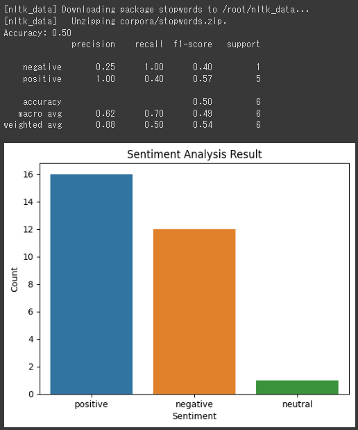
最後に、結果をグラフ化します。

感情ごとの分類数を棒グラフで表示します。

sns.countplot(x='sentiment', data=df)
plt.xlabel('Sentiment')
plt.ylabel('Count')
plt.title('Sentiment Analysis Result')
plt.show()

これにより、ソーシャルメディア感情分析のモデルの予測結果を視覚化できます。

棒グラフで表示される感情のカウントを確認することができます。

[実行結果]

ソースコード解説

このコードは、感情分析（Sentiment Analysis）を行うためのプログラムです。

感情分析は、テキストデータから感情や意見を抽出するための自然言語処理の一種です。

---

まず、必要なライブラリをインポートしています。

numpyは数値計算を行うためのライブラリ、pandasはデータ解析を行うためのライブラリ、matplotlibとseabornはデータの可視化を行うためのライブラリです。

また、テキストの前処理に使用するためにreとnltkもインポートしています。

---

次に、感情分析のためのデータを定義しています。

dataという辞書型の変数に、テキストと感情のペアを格納しています。

このデータは、感情分析のためのトレーニングデータとして使用されます。

その後、pandasのDataFrameオブジェクトを使用して、データを表形式で扱えるようにしています。

DataFrameは、行と列からなるデータ構造で、この場合はテキストと感情の2つの列があります。

---

次に、テキストの前処理を行うための関数preprocess_textを定義しています。

この関数では、テキストから不要な文字を削除し、小文字に変換し、ストップワード（一般的な単語や語句）を除外しています。

これにより、テキストデータをより扱いやすい形式に変換します。

その後、preprocess_text関数をapplyメソッドを使ってデータフレームのtext列に適用し、テキストの前処理を行っています。

---

次に、CountVectorizerクラスを使用してテキストデータをベクトル化しています。

CountVectorizerは、テキストデータを単語の出現回数を表すベクトルに変換するためのクラスです。

fit_transformメソッドを使用することで、テキストデータをベクトル化しています。

その後、データをトレーニングデータとテストデータに分割しています。

train_test_split関数を使用することで、データを指定した割合で分割することができます。

---

次に、MultinomialNBクラスを使用してナイーブベイズ分類器を作成し、トレーニングデータを用いてモデルを学習させています。

学習が完了したら、テストデータを用いて予測を行い、予測結果の正確さを評価しています。

accuracy_score関数を使用することで、予測結果の正確さを計算しています。

また、classification_report関数を使用することで、クラスごとの適合率、再現率、F1スコアなどの評価指標を表示しています。

最後に、感情のカウントを可視化するために、seabornのcountplot関数を使用して棒グラフを作成し、matplotlibを使用してグラフを表示しています。

これにより、各感情の出現回数を視覚的に確認することができます。

---

このコードは、テキストデータから感情を分析し、予測するための基本的な手法を示しています。

感情分析は、レビューやソーシャルメディアの投稿など、さまざまな応用分野で活用されています。

結果解説

以下にそれぞれの指標を説明します。

1. Accuracy (正解率): 0.50

正解率は、全体の予測のうち、正しく分類されたサンプルの割合を示します。
この場合、正解率は50%です。
つまり、テストセットの6つのツイートのうち、3つが正しく分類され、3つが間違って分類されました。

2. Precision (適合率):

適合率は、モデルがポジティブ（positive）と予測したサンプルのうち、実際にポジティブだったサンプルの割合を示します。
negative（ネガティブ）に関しては25%の適合率で、positive（ポジティブ）に関しては100%の適合率です。
つまり、negativeの予測は1つだけ正確であり、positiveの予測は全て正確でした。

3. Recall (再現率):

再現率は、実際にポジティブなサンプルのうち、モデルがポジティブと予測したサンプルの割合を示します。
negativeに関しては100%の再現率で、positiveに関しては40%の再現率です。
つまり、negativeの全てのサンプルを正確に予測し、positiveのうち40%のサンプルを正確に予測しました。

4. F1-score (F1スコア):

F1スコアは、適合率と再現率の調和平均です。
F1スコアが高いほど、適合率と再現率の両方がバランスよく高いことを示します。
この場合、negativeに関しては0.40のF1スコアで、positiveに関しては0.57のF1スコアです。

5. Support (サポート):

Supportは各クラスのサンプル数を示します。
negativeのサポートは1で、positiveのサポートは5です。
つまり、negativeのテストデータは1つだけで、positiveのテストデータは5つあります。

---

総合的に見ると、この感情分析モデルは、negativeクラスの予測においては一部のサンプルを正確に予測しましたが、positiveクラスの予測には改善の余地があります。

モデルの性能を向上させるためには、データの増加や特徴抽出方法の改善、より高度な機械学習アルゴリズムの使用などが考えられます。

また、評価結果を可視化することで、モデルの性能を把握し、改善点を見つけるのに役立ちます。