ニューラルネットワークが複雑になり学習がうまくいかない場合にはバッチ規格化を行うといいです。
バッチ規格化を使うと途中の結果を整理しながら学習をすることができます。
またバッチ再規格化というものがあり、バッチ規格よりもよい性能を示すとのことなのでこの2つを比較してみます。
まずchainerよりMNISTデータを読み込みます。
1
2
3
4
| import chainer.datasets as ds
train, test = ds.get_mnist()
|
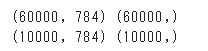
次に読み込んだデータを訓練データとテストデータに分けます。
chainerにはconverくらすにconcat_examplesというメソッドがあり容易にデータの振り分けを行うことができます。
1
2
3
4
5
6
7
8
|
import chainer.dataset.convert as con
xtrain, ttrain = con.concat_examples(train)
xtest, ttest = con.concat_examples(test)
print(xtrain.shape, ttrain.shape)
print(xtest.shape, ttest.shape)
|
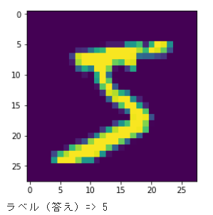
振り分けたデータの1つをmatplotlibを使って表示してみます。
1
2
3
4
5
6
7
8
| import matplotlib.pyplot as plt
Dtrain, N = xtrain.shape
plt.imshow(xtrain[0,:].reshape(28, 28))
plt.show()
print('ラベル(答え)=>', ttrain[0])
|
本題のバッチ規格化を設定します。
まずニューラルネットワークを作成する際にbnorm1=L.BatchNormalization(400)(9行目)を引数に渡し、またニューラルネットワークの関数でNN.bnorm1関数(15行目)をはさみます。
バッチ再規格をする場合は、BatchNormalizationの代わりにBatchRenormalization(10行目)を指定します。
1
2
3
4
5
6
7
8
9
10
11
12
13
14
15
16
17
| import chainer.optimizers as Opt
import chainer.functions as F
import chainer.links as L
from chainer import Variable, Chain, config
C = ttrain.max() + 1
NN = Chain(l1=L.Linear(N, 400), l2=L.Linear(400, C),
bnorm1=L.BatchNormalization(400))
def model(x):
h = NN.l1(x)
h = F.relu(h)
h = NN.bnorm1(h)
h = NN.l2(h)
return h
|
次に学習用関数を定義します。
1
2
3
4
5
6
7
8
9
10
11
12
13
14
15
16
17
18
19
20
21
22
23
24
25
26
27
28
29
30
|
def learning(model, optNN, data, T=50):
train_loss = []
train_acc = []
test_loss = []
test_acc = []
for time in range(T):
config.train = True
optNN.target.zerograds()
ytrain = model(data[0])
loss_train = F.softmax_cross_entropy(ytrain, data[2])
acc_train = F.accuracy(ytrain, data[2])
loss_train.backward()
optNN.update()
config.train = False
ytest = model(data[1])
loss_test = F.softmax_cross_entropy(ytest, data[3])
acc_test = F.accuracy(ytest, data[3])
train_loss.append(loss_train.data)
train_acc.append(acc_train.data)
test_loss.append(loss_test.data)
test_acc.append(acc_test.data)
return train_loss, test_loss, train_acc, test_acc
|
グラフ表示用関数を定義します。
1
2
3
4
5
6
7
8
9
10
11
12
13
14
|
def show_graph(result1, result2, title, xlabel, ylabel, ymin=0.0, ymax=1.0):
Tall = len(result1)
plt.figure(figsize=(8, 6))
plt.plot(range(Tall), result1, label='train')
plt.plot(range(Tall), result2, label='test')
plt.title(title)
plt.xlabel(xlabel)
plt.ylabel(ylabel)
plt.xlim([0, Tall])
plt.ylim(ymin, ymax)
plt.legend()
plt.show()
|
最適化手法を設定し、学習を実行したのち結果をグラフ表示します。
1
2
3
4
5
6
7
8
9
10
|
optNN = Opt.MomentumSGD()
optNN.setup(NN)
train_loss, test_loss, train_acc, test_acc = learning(model, optNN, [xtrain, xtest, ttrain, ttest])
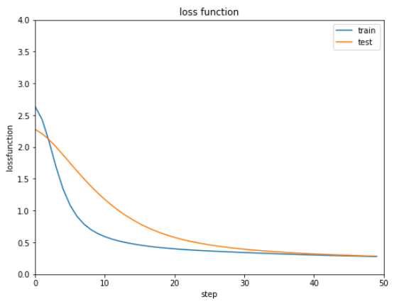
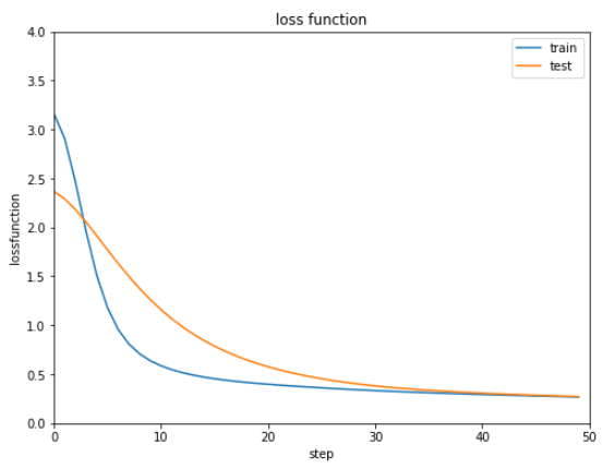
show_graph(train_loss, test_loss, 'loss function', 'step', 'lossfunction', 0.0, 4.0)
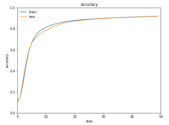
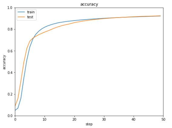
show_graph(train_acc, test_acc, 'accuracy', 'step', 'accuracy')
|
バッチ規格化とバッチ再規格化をそれぞれ実行した結果は下記の通りです。
ほぼ同じ結果で明確な違いがないような気がします。。。
(Google Colaboratoryで動作確認しています。)