ニューラルネットワークで手書き文字の認識をします。有名なMNIST(エムニスト)です。
まず必要なモジュールをインポートします。
1
2
3
4
|
import numpy as np
import matplotlib.pyplot as plt
import sklearn.datasets as ds
|
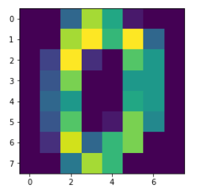
MNISTデータを読み込み、確認のために画像として表示してみます。
1
2
3
4
5
6
7
8
9
10
11
|
MNIST = ds.load_digits()
xdata = MNIST.data.astype(np.float32)
tdata = MNIST.target.astype(np.int32)
D, N = xdata.shape
plt.imshow(xdata[0,:].reshape(8, 8))
plt.show()
|
データ分割関数を定義し、実行します。今回、訓練データと学習データはちょうど半分ずつにしています。
1
2
3
4
5
6
7
8
9
10
11
|
def data_divide(Dtrain, D, xdata, tdata):
index = np.random.permutation(range(D))
xtrain = xdata[index[0:Dtrain],:]
ttrain = tdata[index[0:Dtrain]]
xtest = xdata[index[Dtrain:D],:]
ttest = tdata[index[Dtrain:D]]
return xtrain, xtest, ttrain, ttest
Dtrain = D // 2
xtrain, xtest, ttrain, ttest = data_divide(Dtrain, D, xdata, tdata)
|
chainerの宣言をします。
1
2
3
4
5
|
import chainer.optimizers as Opt
import chainer.functions as F
import chainer.links as L
from chainer import Variable, Chain, config
|
ニューラルネットワークを作成し、ニューラルネットワークの関数を定義します。
また誤差と正解率の遷移を記録する変数を用意します。
1
2
3
4
5
6
7
8
9
10
11
12
13
14
15
16
17
18
19
20
|
C = tdata.max() + 1
NN = Chain(l1=L.Linear(N, 20), l2=L.Linear(20, C))
def model(x):
h = NN.l1(x)
h = F.relu(h)
y = NN.l2(h)
return y
optNN = Opt.MomentumSGD()
optNN.setup(NN)
train_loss = []
train_acc = []
test_loss = []
test_acc = []
|
最適化を行います。今回は200回学習を行います。
1
2
3
4
5
6
7
8
9
10
11
12
13
14
15
16
17
18
19
20
21
22
23
|
T = 200
for time in range(T):
config.train = True
optNN.target.zerograds()
ytrain = model(xtrain)
loss_train = F.softmax_cross_entropy(ytrain, ttrain)
acc_train = F.accuracy(ytrain, ttrain)
loss_train.backward()
optNN.update()
config.train = False
ytest = model(xtest)
loss_test = F.softmax_cross_entropy(ytest, ttest)
acc_test = F.accuracy(ytest, ttest)
train_loss.append(loss_train.data)
test_loss.append(loss_test.data)
train_acc.append(acc_train.data)
test_acc.append(acc_test.data)
|
グラフ表示用の関数を定義します。
1
2
3
4
5
6
7
8
9
10
11
12
13
14
|
def show_graph(result1, result2, title, xlabel, ylabel, ymin=0.0, ymax=1.0):
Tall = len(result1)
plt.figure(figsize=(8, 6))
plt.plot(range(Tall), result1, label='train')
plt.plot(range(Tall), result2, label='test')
plt.title(title)
plt.xlabel(xlabel)
plt.ylabel(ylabel)
plt.xlim([0, Tall])
plt.ylim(ymin, ymax)
plt.legend()
plt.show()
|
誤差と正解率の遷移をグラフ表示します。
1
2
3
|
show_graph(train_loss, test_loss, 'loss function', 'step', 'loss_function', 0.0, 4.0)
show_graph(train_acc, test_acc, 'accuracy', 'step', 'accuracy')
|
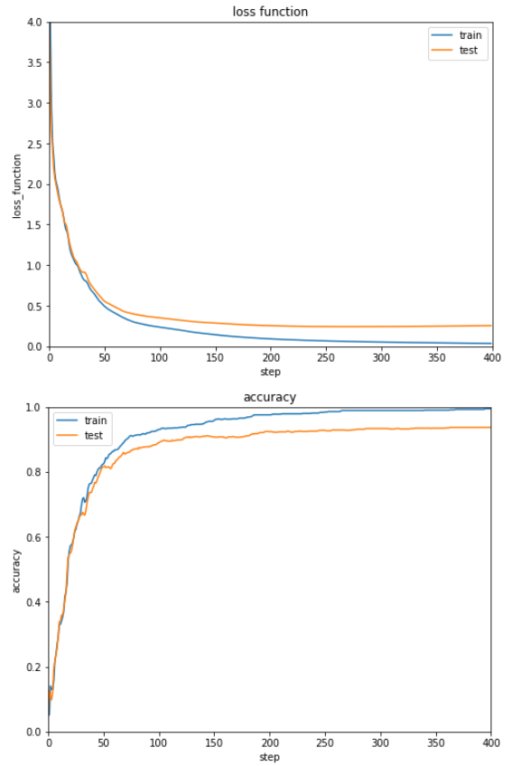
順調に誤差が減少し、正解率が上昇していることが見てとれます。
ただ正解率が9割そこそこなのが少々不満です。
非線形関数や最適化手法を変えて改善する余地はありそうです。
(Google Colaboratoryで動作確認しています。)