いくつかある最適化方法のうち下記の3つを比較します。
まずは必要なモジュールをインポートします。
1
2
3
4
5
6
7
8
| import chainer.optimizers as Opt
import chainer.functions as F
import chainer.links as L
from chainer import Variable, Chain, config
import numpy as np
import matplotlib.pyplot as plt
import sklearn.datasets as ds
|
アヤメデータを読み込み、訓練データと学習データに分けます。
1
2
3
4
5
6
7
8
9
10
11
12
13
14
|
Iris = ds.load_iris()
xdata = Iris.data.astype(np.float32)
tdata = Iris.target.astype(np.int32)
D, N = xdata.shape
Dtrain = D // 2
index = np.random.permutation(range(D))
xtrain = xdata[index[0:Dtrain],:]
ttrain = tdata[index[0:Dtrain]]
xtest = xdata[index[Dtrain:D],:]
ttest = tdata[index[Dtrain:D]]
|
グラフ表示関数を定義します。
1
2
3
4
5
6
7
8
9
10
11
12
13
14
15
16
17
18
19
20
21
22
23
24
25
26
|
def show_graph():
Tall = len(train_loss)
plt.figure(figsize=(8, 6))
plt.plot(range(Tall), train_loss, label='train_loss')
plt.plot(range(Tall), test_loss, label='test_loss')
plt.title('loss function in training and test')
plt.xlabel('step')
plt.ylabel('loss function')
plt.xlim([0, Tall])
plt.ylim(0, 4)
plt.legend()
plt.show()
plt.figure(figsize=(8, 6))
plt.plot(range(Tall), train_acc, label='train_acc')
plt.plot(range(Tall), test_acc, label='test_acc')
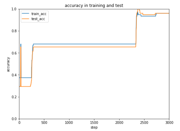
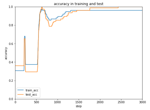
plt.title('accuracy in training and test')
plt.xlabel('step')
plt.ylabel('accuracy')
plt.xlim([0, Tall])
plt.ylim(0, 1.0)
plt.legend()
plt.show()
|
学習用関数を定義します。
1
2
3
4
5
6
7
8
9
10
11
12
13
14
15
16
17
18
19
20
|
def training(T):
for time in range(T):
config.train = True
optNN.target.zerograds()
ytrain = model(xtrain)
loss_train = F.softmax_cross_entropy(ytrain, ttrain)
acc_train = F.accuracy(ytrain, ttrain)
loss_train.backward()
optNN.update()
config.train = False
ytest = model(xtest)
loss_test = F.softmax_cross_entropy(ytest, ttest)
acc_test = F.accuracy(ytest, ttest)
train_loss.append(loss_train.data)
train_acc.append(acc_train.data)
test_loss.append(loss_test.data)
test_acc.append(acc_test.data)
|
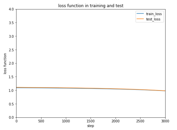
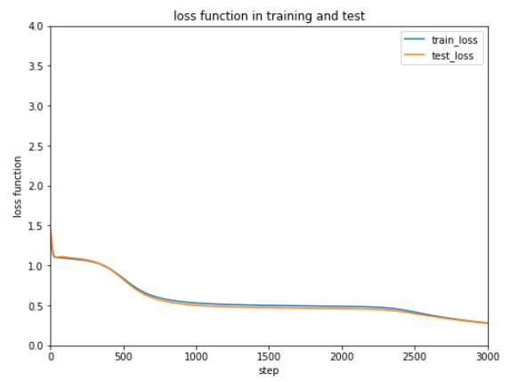
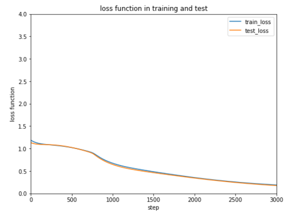
最後に最適化方法を変えながら学習・結果表示を行います。
1
2
3
4
5
6
7
8
9
10
11
12
13
14
15
16
17
18
19
20
21
22
23
24
25
26
27
28
29
30
31
32
|
for optNN in [Opt.SGD(), Opt.MomentumSGD(), Opt.Adam()]:
C = np.max(tdata) + 1
NN = Chain(l1=L.Linear(N, 3), l2=L.Linear(3, 3), l3=L.Linear(3, C))
def model(x):
h = NN.l1(x)
h = F.sigmoid(h)
h = NN.l2(h)
h = F.sigmoid(h)
y = NN.l3(h)
return y
optNN.setup(NN)
train_loss = []
train_acc = []
test_loss = []
test_acc = []
training(3000)
show_graph()
|
実行結果は比較しやすいように表形式にまとめました。
| SGD |
MomentumSGD |
Adam |
| 初歩的な最適化 |
勢いをつけた最適化 |
適応的モーメント勾配法 |
 |
 |
 |
 |
 |
 |
(適応的勾配法は、勾配の大きさが小さくなってくると勾配に従って調整する大きさを多くします。)
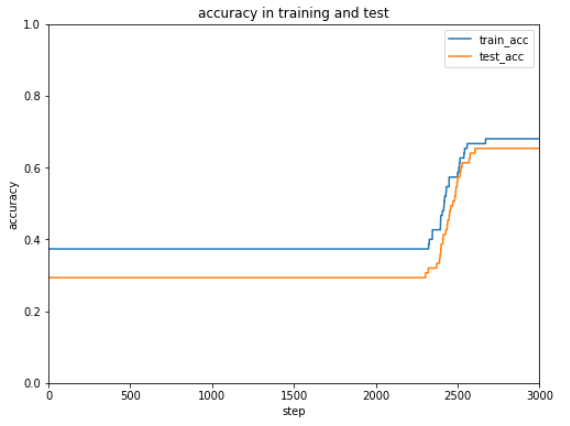
非線形関数にReLUを使用すると実行結果が安定しなかった(すぐ最適化されたりまったくされなかったり・・・)のでシグモイドを使用しています。
今回のケースではAdamが一番はやく正解率が安定しています。
最適化方法によってだいぶ結果が変わるので、データやケースによって最適化方法をいろいろ試すしかなさそうです。。。
(Google Colaboratoryで動作確認しています。)