1
2
3
4
5
6
7
8
9
10
11
12
13
14
15
16
17
18
19
20
21
22
23
24
25
26
27
28
29
30
31
32
33
34
35
36
37
38
39
40
41
42
43
44
45
46
47
48
49
50
51
52
53
54
55
56
57
58
59
60
61
62
63
64
65
66
67
68
69
70
71
72
73
74
75
76
77
78
79
80
81
82
83
84
85
86
87
88
89
90
91
92
93
94
95
96
97
98
99
100
101
102
103
104
105
106
107
108
109
110
111
112
113
114
115
116
117
118
119
120
121
122
123
124
125
126
127
128
129
130
131
132
133
134
135
136
137
138
139
140
141
142
143
144
145
146
147
148
149
150
151
152
153
154
155
156
157
158
159
160
161
162
163
164
165
166
167
168
169
170
171
172
173
174
175
176
177
178
179
180
181
182
183
184
185
186
187
188
189
190
191
192
193
194
195
196
197
198
199
200
201
202
203
204
205
206
207
208
209
210
211
212
213
214
215
216
217
218
219
220
221
222
223
224
225
226
227
228
229
230
231
232
233
234
235
236
237
238
239
240
241
242
243
244
245
246
247
248
249
250
251
252
253
254
255
256
257
258
259
260
261
262
263
264
265
266
267
268
269
270
271
272
273
274
275
276
277
278
279
280
281
282
283
284
285
286
287
288
289
290
291
292
293
294
295
296
297
298
299
300
301
302
303
304
305
306
307
308
309
310
311
312
313
314
315
316
317
318
319
320
321
322
323
324
325
326
327
328
329
330
331
332
333
334
335
336
337
338
339
340
341
342
343
344
345
346
347
348
349
350
351
352
353
354
355
356
357
358
359
360
361
362
363
364
365
366
367
368
369
| import numpy as np
import matplotlib.pyplot as plt
from scipy.optimize import minimize_scalar, minimize
from mpl_toolkits.mplot3d import Axes3D
import warnings
warnings.filterwarnings('ignore')
class NVCenterMagnetometer:
"""
Nitrogen-Vacancy center magnetometer simulation for quantum sensing optimization
"""
def __init__(self, gamma=2.8e10, contrast=0.3, photon_rate=1e6, dead_time=1e-6):
"""
Initialize NV center parameters
Parameters:
- gamma: gyromagnetic ratio (Hz/T) for NV centers
- contrast: signal contrast (dimensionless)
- photon_rate: photon collection rate (Hz)
- dead_time: dead time between measurements (s)
"""
self.gamma = gamma
self.contrast = contrast
self.photon_rate = photon_rate
self.dead_time = dead_time
def signal_amplitude(self, B, t):
"""
Calculate signal amplitude for given magnetic field and measurement time
S = A * sin(gamma * B * t)
For small fields: S ≈ A * gamma * B * t
"""
return self.contrast * self.gamma * B * t
def shot_noise(self, t):
"""
Calculate shot noise limited by photon statistics
σ = 1/√N where N is number of photons collected
"""
N_photons = self.photon_rate * t
return 1.0 / np.sqrt(N_photons)
def precision_single_measurement(self, B, t):
"""
Calculate precision for a single measurement
Precision = |dS/dB| / σ_noise
"""
signal_derivative = self.contrast * self.gamma * t
noise = self.shot_noise(t)
return signal_derivative / noise
def precision_repeated_measurements(self, B, t, n_measurements):
"""
Calculate precision for repeated measurements
Precision scales as √n for independent measurements
"""
single_precision = self.precision_single_measurement(B, t)
return single_precision * np.sqrt(n_measurements)
def total_time_constraint(self, t, n_measurements):
"""
Calculate total time including dead time
T_total = n * (t + t_dead)
"""
return n_measurements * (t + self.dead_time)
def optimize_for_fixed_total_time(self, B, total_time):
"""
Optimize measurement time and repetitions for fixed total measurement time
"""
def negative_precision(t):
if t <= 0 or t >= total_time:
return 1e10
n_max = int(total_time / (t + self.dead_time))
if n_max <= 0:
return 1e10
precision = self.precision_repeated_measurements(B, t, n_max)
return -precision
result = minimize_scalar(negative_precision, bounds=(1e-6, total_time-1e-6), method='bounded')
optimal_t = result.x
optimal_n = int(total_time / (optimal_t + self.dead_time))
optimal_precision = -result.fun
return optimal_t, optimal_n, optimal_precision
def ramsey_sequence_precision(self, B, tau, n_measurements):
"""
Calculate precision for Ramsey interferometry sequence
More sophisticated pulse sequence with enhanced sensitivity
"""
phase = self.gamma * B * tau
signal = self.contrast * np.sin(phase)
if abs(phase) < 0.1:
signal_derivative = self.contrast * self.gamma * tau
else:
signal_derivative = self.contrast * self.gamma * tau * np.cos(phase)
total_measurement_time = 2 * 1e-6 + tau
noise = self.shot_noise(total_measurement_time)
precision = abs(signal_derivative) / noise * np.sqrt(n_measurements)
return precision
nv_mag = NVCenterMagnetometer(
gamma=2.8e10,
contrast=0.3,
photon_rate=1e6,
dead_time=1e-6
)
B_field = 1e-9
print("=== Quantum Sensing Optimization Analysis ===\n")
measurement_times = np.logspace(-6, -3, 100)
single_precisions = [nv_mag.precision_single_measurement(B_field, t) for t in measurement_times]
print("1. Single Measurement Analysis:")
print(f" Target magnetic field: {B_field*1e9:.1f} nT")
print(f" Measurement time range: {measurement_times[0]*1e6:.1f} μs to {measurement_times[-1]*1e3:.1f} ms")
total_times = [1e-3, 5e-3, 10e-3, 50e-3, 100e-3]
optimization_results = []
print("\n2. Optimization Results for Different Time Budgets:")
print(" Total Time | Optimal t | Optimal n | Max Precision | Sensitivity")
print(" -----------|-----------|-----------|---------------|------------")
for T_total in total_times:
opt_t, opt_n, opt_precision = nv_mag.optimize_for_fixed_total_time(B_field, T_total)
sensitivity = 1.0 / opt_precision
optimization_results.append((T_total, opt_t, opt_n, opt_precision, sensitivity))
print(f" {T_total*1e3:6.1f} ms |{opt_t*1e6:8.1f} μs |{opt_n:8d} |{opt_precision:.2e} |{sensitivity*1e12:.2f} pT/√Hz")
ramsey_times = np.logspace(-6, -4, 50)
ramsey_precisions = []
n_ramsey = 1000
print(f"\n3. Ramsey Interferometry Analysis (n = {n_ramsey} sequences):")
for tau in ramsey_times:
precision = nv_mag.ramsey_sequence_precision(B_field, tau, n_ramsey)
ramsey_precisions.append(precision)
optimal_ramsey_idx = np.argmax(ramsey_precisions)
optimal_tau = ramsey_times[optimal_ramsey_idx]
optimal_ramsey_precision = ramsey_precisions[optimal_ramsey_idx]
print(f" Optimal free evolution time: {optimal_tau*1e6:.1f} μs")
print(f" Maximum Ramsey precision: {optimal_ramsey_precision:.2e}")
print(f" Ramsey sensitivity: {1.0/optimal_ramsey_precision*1e12:.2f} pT/√Hz")
print("\n4. Parameter Sensitivity Analysis:")
contrasts = np.linspace(0.1, 0.8, 8)
contrast_precisions = []
for c in contrasts:
nv_temp = NVCenterMagnetometer(contrast=c)
_, _, precision = nv_temp.optimize_for_fixed_total_time(B_field, 10e-3)
contrast_precisions.append(precision)
print(f" Contrast range: {contrasts[0]:.1f} to {contrasts[-1]:.1f}")
print(f" Precision improvement: {contrast_precisions[-1]/contrast_precisions[0]:.1f}x")
photon_rates = np.logspace(5, 7, 8)
rate_precisions = []
for rate in photon_rates:
nv_temp = NVCenterMagnetometer(photon_rate=rate)
_, _, precision = nv_temp.optimize_for_fixed_total_time(B_field, 10e-3)
rate_precisions.append(precision)
print(f" Photon rate range: {photon_rates[0]:.0e} to {photon_rates[-1]:.0e} Hz")
print(f" Precision improvement: {rate_precisions[-1]/rate_precisions[0]:.1f}x")
print("\n=== Analysis Complete ===")
fig = plt.figure(figsize=(16, 12))
plt.style.use('seaborn-v0_8')
ax1 = plt.subplot(2, 3, 1)
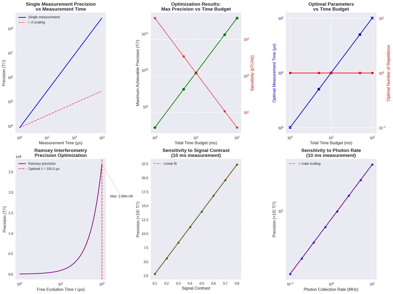
plt.loglog(measurement_times * 1e6, single_precisions, 'b-', linewidth=2, label='Single measurement')
plt.xlabel('Measurement Time (μs)', fontsize=12)
plt.ylabel('Precision (T⁻¹)', fontsize=12)
plt.title('Single Measurement Precision\nvs Measurement Time', fontsize=14, fontweight='bold')
plt.grid(True, alpha=0.3)
plt.legend()
theoretical = single_precisions[0] * (measurement_times / measurement_times[0])**0.5
plt.loglog(measurement_times * 1e6, theoretical, 'r--', alpha=0.7, label='∝ √t scaling')
plt.legend()
ax2 = plt.subplot(2, 3, 2)
total_times_plot = [r[0] for r in optimization_results]
optimal_precisions = [r[3] for r in optimization_results]
plt.loglog(np.array(total_times_plot) * 1e3, optimal_precisions, 'go-', linewidth=2, markersize=8)
plt.xlabel('Total Time Budget (ms)', fontsize=12)
plt.ylabel('Maximum Achievable Precision (T⁻¹)', fontsize=12)
plt.title('Optimization Results:\nMax Precision vs Time Budget', fontsize=14, fontweight='bold')
plt.grid(True, alpha=0.3)
ax2_twin = ax2.twinx()
sensitivities = [1.0/p * 1e12 for p in optimal_precisions]
ax2_twin.loglog(np.array(total_times_plot) * 1e3, sensitivities, 'ro-', alpha=0.7)
ax2_twin.set_ylabel('Sensitivity (pT/√Hz)', fontsize=12, color='red')
ax2_twin.tick_params(axis='y', labelcolor='red')
ax3 = plt.subplot(2, 3, 3)
optimal_t_values = [r[1] * 1e6 for r in optimization_results]
optimal_n_values = [r[2] for r in optimization_results]
ax3.loglog(np.array(total_times_plot) * 1e3, optimal_t_values, 'bs-', linewidth=2, label='Optimal t (μs)')
ax3.set_xlabel('Total Time Budget (ms)', fontsize=12)
ax3.set_ylabel('Optimal Measurement Time (μs)', fontsize=12, color='blue')
ax3.tick_params(axis='y', labelcolor='blue')
ax3_twin = ax3.twinx()
ax3_twin.loglog(np.array(total_times_plot) * 1e3, optimal_n_values, 'ro-', linewidth=2, label='Optimal n')
ax3_twin.set_ylabel('Optimal Number of Repetitions', fontsize=12, color='red')
ax3_twin.tick_params(axis='y', labelcolor='red')
plt.title('Optimal Parameters\nvs Time Budget', fontsize=14, fontweight='bold')
ax4 = plt.subplot(2, 3, 4)
plt.semilogx(ramsey_times * 1e6, ramsey_precisions, 'purple', linewidth=2, label='Ramsey precision')
plt.axvline(optimal_tau * 1e6, color='red', linestyle='--', alpha=0.8, label=f'Optimal τ = {optimal_tau*1e6:.1f} μs')
plt.xlabel('Free Evolution Time τ (μs)', fontsize=12)
plt.ylabel('Precision (T⁻¹)', fontsize=12)
plt.title('Ramsey Interferometry\nPrecision Optimization', fontsize=14, fontweight='bold')
plt.grid(True, alpha=0.3)
plt.legend()
plt.annotate(f'Max: {optimal_ramsey_precision:.2e}',
xy=(optimal_tau * 1e6, optimal_ramsey_precision),
xytext=(optimal_tau * 1e6 * 3, optimal_ramsey_precision * 0.7),
arrowprops=dict(arrowstyle='->', color='red', alpha=0.7),
fontsize=10, ha='center')
ax5 = plt.subplot(2, 3, 5)
plt.plot(contrasts, np.array(contrast_precisions)/1e9, 'go-', linewidth=2, markersize=6)
plt.xlabel('Signal Contrast', fontsize=12)
plt.ylabel('Precision (×10⁹ T⁻¹)', fontsize=12)
plt.title('Sensitivity to Signal Contrast\n(10 ms measurement)', fontsize=14, fontweight='bold')
plt.grid(True, alpha=0.3)
z = np.polyfit(contrasts, contrast_precisions, 1)
p = np.poly1d(z)
plt.plot(contrasts, p(contrasts)/1e9, 'r--', alpha=0.7, label='Linear fit')
plt.legend()
ax6 = plt.subplot(2, 3, 6)
plt.loglog(photon_rates/1e6, np.array(rate_precisions)/1e9, 'bo-', linewidth=2, markersize=6)
plt.xlabel('Photon Collection Rate (MHz)', fontsize=12)
plt.ylabel('Precision (×10⁹ T⁻¹)', fontsize=12)
plt.title('Sensitivity to Photon Rate\n(10 ms measurement)', fontsize=14, fontweight='bold')
plt.grid(True, alpha=0.3)
sqrt_scaling = rate_precisions[0] * np.sqrt(photon_rates / photon_rates[0])
plt.loglog(photon_rates/1e6, sqrt_scaling/1e9, 'r--', alpha=0.7, label='∝ √rate scaling')
plt.legend()
plt.tight_layout()
plt.show()
fig2 = plt.figure(figsize=(12, 5))
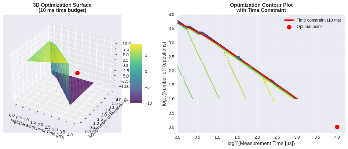
ax_3d = fig2.add_subplot(121, projection='3d')
t_range = np.logspace(-6, -3, 30)
n_range = np.logspace(1, 4, 30)
T_mesh, N_mesh = np.meshgrid(t_range, n_range)
total_time_budget = 10e-3
Z_mesh = np.zeros_like(T_mesh)
for i in range(len(n_range)):
for j in range(len(t_range)):
t = t_range[j]
n = n_range[i]
total_time = n * (t + nv_mag.dead_time)
if total_time <= total_time_budget:
Z_mesh[i, j] = nv_mag.precision_repeated_measurements(B_field, t, n)
else:
Z_mesh[i, j] = 0
surf = ax_3d.plot_surface(np.log10(T_mesh * 1e6), np.log10(N_mesh), np.log10(Z_mesh + 1e-10),
cmap='viridis', alpha=0.8, linewidth=0, antialiased=True)
ax_3d.set_xlabel('log₁₀(Measurement Time [μs])', fontsize=10)
ax_3d.set_ylabel('log₁₀(Number of Repetitions)', fontsize=10)
ax_3d.set_zlabel('log₁₀(Precision [T⁻¹])', fontsize=10)
ax_3d.set_title('3D Optimization Surface\n(10 ms time budget)', fontsize=12, fontweight='bold')
opt_t_10ms, opt_n_10ms, opt_prec_10ms = nv_mag.optimize_for_fixed_total_time(B_field, 10e-3)
ax_3d.scatter([np.log10(opt_t_10ms * 1e6)], [np.log10(opt_n_10ms)], [np.log10(opt_prec_10ms)],
color='red', s=100, label='Optimal point')
plt.colorbar(surf, shrink=0.5, aspect=5)
ax_2d = fig2.add_subplot(122)
contour = ax_2d.contour(np.log10(T_mesh * 1e6), np.log10(N_mesh), np.log10(Z_mesh + 1e-10),
levels=20, cmap='viridis')
ax_2d.clabel(contour, inline=True, fontsize=8, fmt='%.1f')
t_constraint = np.logspace(-6, -3, 100)
n_constraint = total_time_budget / (t_constraint + nv_mag.dead_time)
valid_mask = n_constraint >= 1
ax_2d.plot(np.log10(t_constraint[valid_mask] * 1e6), np.log10(n_constraint[valid_mask]),
'r-', linewidth=3, label='Time constraint (10 ms)')
ax_2d.scatter([np.log10(opt_t_10ms * 1e6)], [np.log10(opt_n_10ms)],
color='red', s=100, zorder=5, label='Optimal point')
ax_2d.set_xlabel('log₁₀(Measurement Time [μs])', fontsize=12)
ax_2d.set_ylabel('log₁₀(Number of Repetitions)', fontsize=12)
ax_2d.set_title('Optimization Contour Plot\nwith Time Constraint', fontsize=12, fontweight='bold')
ax_2d.legend()
ax_2d.grid(True, alpha=0.3)
plt.tight_layout()
plt.show()
print("\n=== Visualization Complete ===")
print(f"Key findings from optimization:")
print(f"• Single measurement precision scales as √t")
print(f"• Repeated measurements improve precision by √n")
print(f"• Dead time creates trade-off between individual and repeated measurements")
print(f"• Optimal strategy depends on total time budget")
print(f"• Ramsey interferometry provides enhanced sensitivity for specific evolution times")
print(f"• System performance scales linearly with contrast and as √(photon rate)")
|