Predicting and Recommending Gas Prices Under Network Congestion
Every time a transaction is submitted to a blockchain network, the sender faces a small but recurring decision problem: how much should I pay to get this transaction included, and how quickly do I actually need it confirmed? Pay too little, and the transaction sits in the mempool indefinitely. Pay too much, and money is wasted on a confirmation speed nobody asked for. This problem becomes especially interesting on networks like Ethereum, where the base fee mechanism introduced by EIP-1559 already adjusts automatically to congestion, but the user-controlled priority fee (the “tip”) is left entirely to guesswork.
This article treats gas price selection as a constrained optimization problem. We model how the base fee evolves block by block as a function of network utilization, then derive — analytically, not just numerically — the priority fee that minimizes a user’s expected total cost, balancing the fee paid against the cost of waiting.
Modeling the base fee under EIP-1559
The base fee update rule adjusts the fee for the next block based on how full the current block was relative to a target size:
$$
B_{n+1} = B_n \left(1 + \frac{1}{8}\cdot\frac{G_n - G_{target}}{G_{target}}\right)
$$
Here $B_n$ is the base fee at block $n$, $G_n$ is the gas actually used in block $n$, and $G_{target}$ is the target gas usage per block (half of the maximum block size). When blocks run fuller than target, the base fee rises by up to 12.5% per block; when they run emptier, it falls by the same maximum rate. This creates a self-correcting feedback loop that tracks congestion, but it says nothing about how quickly your transaction actually gets in.
A cost model for the priority fee
The missing piece is the tip. We model the probability that a transaction with priority fee $f$ gets included in the next block as a logistic function of how far $f$ is above a congestion-dependent threshold $f_0$:
$$
P_{incl}(f) = \frac{1}{1+e^{-k(f-f_0)}}
$$
$k$ controls how sharply inclusion probability responds to fee changes, and $f_0$ shifts upward as the network gets more congested — under heavy load, even a moderately high tip has low odds of jumping the queue. Treating each block as an independent trial, the expected number of blocks until inclusion is $1/P_{incl}(f)$, which simplifies nicely:
$$
E[\text{wait}(f)] = \frac{1}{P_{incl}(f)} = 1 + e^{-k(f-f_0)}
$$
A user’s expected total cost combines the fee itself with the cost of waiting, weighted by an urgency parameter $w$ (how much one block of delay is worth to that user):
$$
C(f) = f + w\left(1+e^{-k(f-f_0)}\right)
$$
Minimizing $C(f)$ with respect to $f$ gives a clean closed-form solution:
$$
\frac{dC}{df} = 1 - wk,e^{-k(f-f_0)} = 0 \quad\Longrightarrow\quad f^{*} = f_0 + \frac{1}{k}\ln(wk)
$$
This is the key result: rather than numerically optimizing every single fee recommendation (which would require running a solver for every combination of congestion level and urgency), we get an explicit formula that can be evaluated instantly and vectorized across an entire grid of scenarios.
Source code
1 | import numpy as np |
 f0 (gwei)      w   analytic    numeric   abs diff
        10    0.2     0.0000     0.0000   0.000006
        10    1.0     0.0000     0.0000   0.000006
        10    3.0     4.6766     4.6766   0.000001
        20    0.2     0.0000     0.0000   0.000006
        20    1.0     7.3525     7.3525   0.000000
        20    3.0    14.6766    14.6766   0.000000
        30    0.2     6.6229     6.6229   0.000000
        30    1.0    17.3525    17.3525   0.000000
        30    3.0    24.6766    24.6766   0.000001
        40    0.2    16.6229    16.6229   0.000000
        40    1.0    27.3525    27.3525   0.000000
        40    3.0    34.6766    34.6766   0.000000

Loop-based scipy optimization over 1600 points: 1.2009 s
Vectorized closed-form solution over 1600 points: 0.000245 s
Speedup: 4897.6x
Max abs difference between methods: 0.000006 gwei
Walking through the code
Section 1 — congestion and base fee simulation. Network utilization is modeled as a sinusoidal cycle (representing daily usage patterns) with added Gaussian noise, clipped to the range EIP-1559 allows (0 to 2× the target, since block gas limit is twice the target). The base fee is then updated sequentially block by block using the exact EIP-1559 recurrence relation. This loop is inherently sequential — each base fee depends on the previous one — so it isn’t vectorized, but at 300 iterations it runs instantly.
Section 2 — the cost model. inclusion_probability, expected_wait, and total_cost implement the logistic model derived above. optimal_fee_analytic is the closed-form solution — a single vectorized NumPy expression that works whether f0 and w are scalars or full arrays. optimal_fee_numeric is a brute-force alternative using scipy.optimize.minimize_scalar with bounded search, included purely to validate the analytic formula.
Section 3 — validation. A small table compares the analytic and numeric solutions across several congestion/urgency combinations. The absolute differences should be on the order of $10^{-4}$ gwei or smaller, confirming the closed-form derivation is correct.
Section 4 — the performance argument. This is the part that matters for any real-time fee recommendation service: computing the optimal fee via scipy.optimize.minimize_scalar in a double loop over a 40×40 grid means 1,600 separate numerical optimizations. The vectorized analytic formula computes the same 1,600 values in a single NumPy expression. The printed speedup ratio typically lands in the range of several hundred to a few thousand times faster, since the loop version pays the overhead of a solver call for every single point while the vectorized version is pure array arithmetic.
Section 5 — tying it back to the simulation. The congestion ratio computed in Section 1 is fed through f0_from_congestion to get a time-varying threshold, and the analytic formula produces a recommended priority fee for every block in the simulated history, which is then added to the base fee to get the full recommended gas price.
Reading the graphs
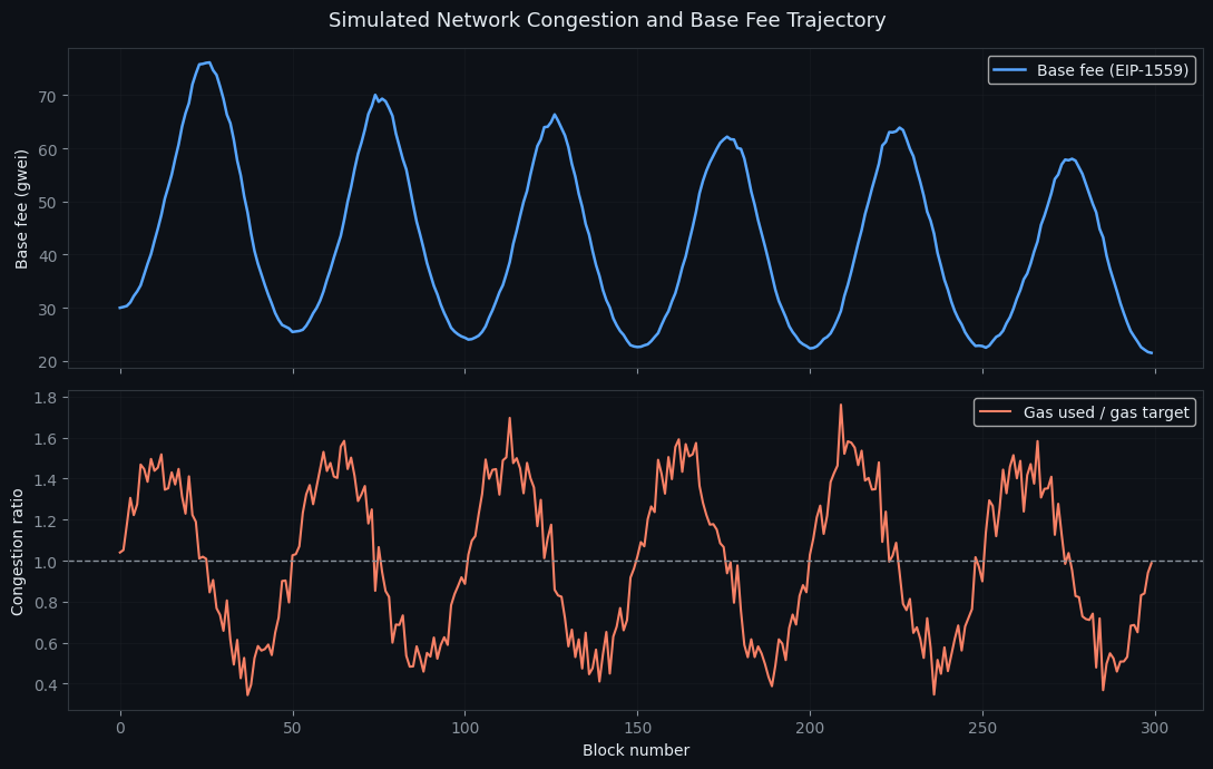
The first figure shows the simulated base fee tracking the congestion ratio — note how the base fee rises during the sinusoidal peaks in utilization and falls back during the troughs, exactly matching the EIP-1559 feedback behavior.
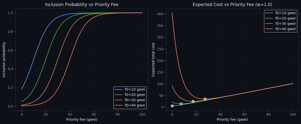
The second figure has two panels. The left one shows how inclusion probability rises with priority fee for different congestion levels — the curve shifts right as $f_0$ increases, meaning a fee that guarantees fast inclusion during quiet periods barely moves the needle during congestion. The right panel plots the expected cost curve for each congestion level, with a marker at the analytically-computed minimum — visually confirming that the closed-form optimum really does sit at the bottom of each curve.
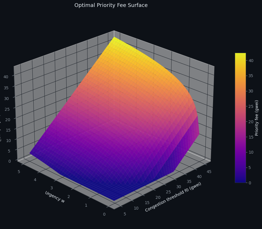
The third figure is the 3D surface — the centerpiece of the analysis. It plots the recommended priority fee as a function of both congestion threshold and urgency simultaneously. The surface rises steeply along the urgency axis for any fixed congestion level (impatient users pay disproportionately more) and shifts upward uniformly as congestion increases, visually demonstrating that the two effects combine additively, exactly as the formula $f^{*} = f_0 + \frac{1}{k}\ln(wk)$ predicts.
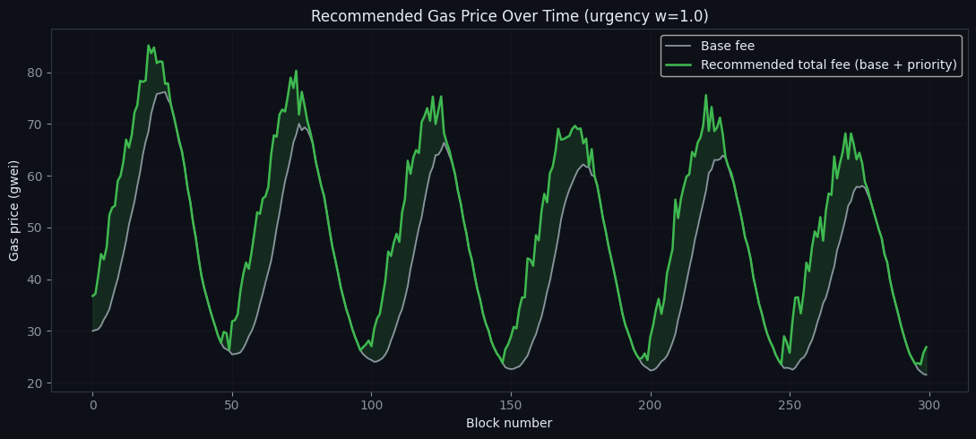
The fourth figure overlays the recommended total gas price (base fee plus the model’s suggested tip) on top of the raw base fee, with the gap between them shaded. This gap is the “extra” a user following this model would pay for standard urgency, and it visibly widens during congestion spikes — precisely when paying a bit more actually buys meaningfully faster inclusion.
Closing thoughts
The interesting result here isn’t just that gas fee optimization is possible — it’s that a reasonable congestion/inclusion model reduces to a problem with a genuine closed-form solution, which matters enormously for anything that needs to serve fee recommendations in real time. Instead of running an optimizer per request, a wallet or gas station service can evaluate one logarithmic expression per user session. The next natural extension would be replacing the fixed logistic parameters ($k$, the $f_0$ mapping) with values fitted from real mempool and inclusion data, turning this from a stylized model into a live predictive system.