Fréchet Mean (Karcher Mean) on Riemannian Manifolds

A Hands-On Python Tutorial

The concept of “average” is intuitive in flat Euclidean space — just add up the vectors and divide. But what happens when your data lives on a curved surface, like a sphere? The straight-line mean may not even lie on the manifold. This is where the Fréchet mean (also called the Karcher mean) steps in, generalizing the notion of a mean to Riemannian geometry.


What Is the Fréchet Mean?

Given a set of points ${x_1, x_2, \ldots, x_n}$ on a Riemannian manifold $(\mathcal{M}, g)$, the Fréchet mean is defined as the point $\mu^* \in \mathcal{M}$ that minimizes the sum of squared geodesic distances:

$$
\mu^* = \arg\min_{\mu \in \mathcal{M}} \sum_{i=1}^{n} d_{\mathcal{M}}(\mu, x_i)^2
$$

where $d_{\mathcal{M}}(\cdot, \cdot)$ is the geodesic distance on the manifold.

In Euclidean space $\mathbb{R}^n$, geodesics are straight lines and $d(x, y) = |x - y|$, so the Fréchet mean reduces to the ordinary arithmetic mean.


The Algorithm: Riemannian Gradient Descent

The Karcher mean algorithm uses Riemannian gradient descent via the exponential and logarithmic maps:

  1. Initialize $\mu_0 \in \mathcal{M}$
  2. At each step $t$, compute the Riemannian gradient:

$$
\text{grad} F(\mu_t) = -\frac{2}{n} \sum_{i=1}^{n} \log_{\mu_t}(x_i)
$$

  1. Update via the exponential map:

$$
\mu_{t+1} = \exp_{\mu_t}!\left(\frac{1}{n} \sum_{i=1}^{n} \log_{\mu_t}(x_i)\right)
$$

  1. Repeat until convergence: $|\bar{v}_t| < \varepsilon$

Concrete Example: Points on the 2-Sphere $S^2$

We will work on the unit sphere $S^2 \subset \mathbb{R}^3$. This is one of the most natural and important Riemannian manifolds, appearing in directional statistics, computer vision, and robotics.

Key Maps on $S^2$

Exponential map at $p$, tangent vector $v \in T_p S^2$:

$$
\exp_p(v) = \cos(|v|), p + \sin(|v|), \frac{v}{|v|}
$$

Logarithmic map (inverse of exponential) from $p$ to $q$:

$$
\log_p(q) = \frac{\theta}{\sin\theta}\left(q - \cos\theta \cdot p\right), \quad \theta = \arccos(\langle p, q \rangle)
$$

Geodesic distance:

$$
d(p, q) = \arccos(\langle p, q \rangle)
$$


Python Implementation

1
2
3
4
5
6
7
8
9
10
11
12
13
14
15
16
17
18
19
20
21
22
23
24
25
26
27
28
29
30
31
32
33
34
35
36
37
38
39
40
41
42
43
44
45
46
47
48
49
50
51
52
53
54
55
56
57
58
59
60
61
62
63
64
65
66
67
68
69
70
71
72
73
74
75
76
77
78
79
80
81
82
83
84
85
86
87
88
89
90
91
92
93
94
95
96
97
98
99
100
101
102
103
104
105
106
107
108
109
110
111
112
113
114
115
116
117
118
119
120
121
122
123
124
125
126
127
128
129
130
131
132
133
134
135
136
137
138
139
140
141
142
143
144
145
146
147
148
149
150
151
152
153
154
155
156
157
158
159
160
161
162
163
164
165
166
167
168
169
170
171
172
173
174
175
176
177
178
179
180
181
182
183
184
185
186
187
188
189
190
191
192
193
194
195
196
197
198
199
200
201
202
203
204
205
206
207
208
209
210
211
212
213
214
215
216
217
218
219
220
221
222
223
224
225
226
227
228
229
230
231
232
233
234
235
236
237
238
239
240
241
242
243
244
245
246
247
248
249
250
251
252
253
254
255
256
257
258
259
260
261
262
263
264
265
266
267
268
269
270
271
272
273
274
# ============================================================
# Fréchet Mean (Karcher Mean) on the 2-Sphere S²
# ============================================================

import numpy as np
import matplotlib.pyplot as plt
from mpl_toolkits.mplot3d import Axes3D
from matplotlib import cm
import warnings
warnings.filterwarnings("ignore")

# ── Reproducibility ──────────────────────────────────────────
np.random.seed(42)

# ============================================================
# 1. Core Riemannian Operations on S²
# ============================================================

def normalize(v):
"""Project a vector onto the unit sphere."""
return v / np.linalg.norm(v)

def log_map(p, q):
"""
Logarithmic map at p towards q on S².
Returns the tangent vector at p pointing towards q.
"""
# Clamp inner product to [-1, 1] for numerical stability
inner = np.clip(np.dot(p, q), -1.0, 1.0)
theta = np.arccos(inner)
if theta < 1e-10: # p ≈ q: log is essentially zero
return np.zeros(3)
return (theta / np.sin(theta)) * (q - inner * p)

def exp_map(p, v):
"""
Exponential map at p with tangent vector v on S².
Moves along the geodesic starting at p in direction v.
"""
norm_v = np.linalg.norm(v)
if norm_v < 1e-10:
return p
return np.cos(norm_v) * p + np.sin(norm_v) * (v / norm_v)

def geodesic_distance(p, q):
"""Great-circle distance between p and q on S²."""
inner = np.clip(np.dot(p, q), -1.0, 1.0)
return np.arccos(inner)

# ============================================================
# 2. Karcher Mean Algorithm (Vectorised for Speed)
# ============================================================

def karcher_mean(points, max_iter=500, tol=1e-9):
"""
Compute the Fréchet / Karcher mean of a set of points on S².

Parameters
----------
points : (N, 3) ndarray – unit vectors on S²
max_iter : int – maximum iterations
tol : float – convergence threshold (tangent vector norm)

Returns
-------
mean : (3,) ndarray – Karcher mean
history : list of (3,) – mean at each iteration (for visualisation)
errors : list of float – tangent-vector norms (convergence curve)
"""
# Initialise with the normalised Euclidean mean (good warm start)
mu = normalize(points.mean(axis=0))
history = [mu.copy()]
errors = []

for _ in range(max_iter):
# Tangent vectors from current estimate to each data point
logs = np.array([log_map(mu, q) for q in points]) # (N, 3)
mean_log = logs.mean(axis=0) # (3,)

err = np.linalg.norm(mean_log)
errors.append(err)

if err < tol:
break

mu = normalize(exp_map(mu, mean_log))
history.append(mu.copy())

return mu, history, errors

# ============================================================
# 3. Generate Synthetic Data on S²
# ============================================================

def random_point_on_sphere():
"""Uniformly sample a point on S²."""
v = np.random.randn(3)
return normalize(v)

def perturb_point(p, sigma=0.3):
"""
Add a small random tangent perturbation to p,
then project back onto S².
"""
# Random tangent vector (perpendicular to p)
v = np.random.randn(3)
v -= np.dot(v, p) * p # project out the normal component
v = v / np.linalg.norm(v) * np.random.rayleigh(sigma)
return normalize(exp_map(p, v))

# True mean (ground truth) — a nice canonical point
true_mean = normalize(np.array([1.0, 1.0, 1.0]))

# 30 noisy observations scattered around the true mean
N = 30
points = np.array([perturb_point(true_mean, sigma=0.4) for _ in range(N)])

# ============================================================
# 4. Compute the Karcher Mean
# ============================================================

karcher_mu, history, errors = karcher_mean(points, max_iter=500, tol=1e-10)
history = np.array(history)

print("=" * 50)
print(f"True mean (normalised): {true_mean}")
print(f"Karcher mean: {karcher_mu}")
print(f"Geodesic error: {geodesic_distance(true_mean, karcher_mu):.6f} rad")
print(f"Converged in {len(errors)} iterations")
print("=" * 50)

# ============================================================
# 5. Visualisation
# ============================================================

# ── Helper: draw a wireframe sphere ─────────────────────────
def sphere_mesh(n=60):
u = np.linspace(0, 2 * np.pi, n)
v = np.linspace(0, np.pi, n)
x = np.outer(np.cos(u), np.sin(v))
y = np.outer(np.sin(u), np.sin(v))
z = np.outer(np.ones(n), np.cos(v))
return x, y, z

fig = plt.figure(figsize=(18, 13))
fig.patch.set_facecolor('#0d1117')

# ── Panel 1: 3-D Sphere with data, true mean, Karcher mean ──
ax1 = fig.add_subplot(221, projection='3d')
ax1.set_facecolor('#0d1117')

sx, sy, sz = sphere_mesh()
ax1.plot_surface(sx, sy, sz, alpha=0.08, color='#4a9eff',
linewidth=0, antialiased=True)
ax1.plot_wireframe(sx, sy, sz, alpha=0.05, color='#4a9eff', linewidth=0.3)

# Data points
ax1.scatter(points[:, 0], points[:, 1], points[:, 2],
color='#ff6b6b', s=35, alpha=0.9, label='Data points', zorder=5)

# Karcher mean iteration path
ax1.plot(history[:, 0], history[:, 1], history[:, 2],
color='#ffd700', linewidth=1.5, alpha=0.7, label='Karcher path')
ax1.scatter(*history[0], color='#ff9f43', s=80, marker='^',
zorder=6, label='Init')

# True mean
ax1.scatter(*true_mean, color='#00ff88', s=120, marker='*',
zorder=7, label='True mean', edgecolors='white', linewidth=0.5)

# Karcher mean
ax1.scatter(*karcher_mu, color='#ffd700', s=150, marker='D',
zorder=8, label='Karcher mean', edgecolors='white', linewidth=0.5)

ax1.set_title('S² Data & Karcher Mean', color='white', fontsize=13, pad=10)
ax1.tick_params(colors='#888888', labelsize=7)
for pane in [ax1.xaxis.pane, ax1.yaxis.pane, ax1.zaxis.pane]:
pane.fill = False
pane.set_edgecolor('#333333')
ax1.legend(loc='upper left', fontsize=7, framealpha=0.3,
labelcolor='white', facecolor='#1a1a2e')

# ── Panel 2: Convergence curve ───────────────────────────────
ax2 = fig.add_subplot(222)
ax2.set_facecolor('#0d1117')
ax2.semilogy(errors, color='#4a9eff', linewidth=2)
ax2.fill_between(range(len(errors)), errors,
alpha=0.15, color='#4a9eff')
ax2.axhline(1e-10, color='#ffd700', linestyle='--',
linewidth=1, label='Tolerance $10^{-10}$')
ax2.set_xlabel('Iteration', color='#aaaaaa')
ax2.set_ylabel(r'$\|\bar{v}\|$ (tangent norm)', color='#aaaaaa')
ax2.set_title('Convergence of Karcher Mean', color='white', fontsize=13)
ax2.tick_params(colors='#888888')
ax2.spines[:].set_color('#333333')
ax2.legend(fontsize=9, framealpha=0.3,
labelcolor='white', facecolor='#1a1a2e')
ax2.grid(alpha=0.15, color='#444444')

# ── Panel 3: Geodesic distances from Karcher mean ────────────
ax3 = fig.add_subplot(223)
ax3.set_facecolor('#0d1117')

dists_karcher = np.array([geodesic_distance(karcher_mu, q) for q in points])
dists_eucl_mean = np.array([
geodesic_distance(normalize(points.mean(axis=0)), q)
for q in points
])

idx = np.arange(N)
ax3.bar(idx - 0.2, dists_eucl_mean, width=0.35, color='#ff6b6b',
alpha=0.8, label='Euclidean mean (projected)')
ax3.bar(idx + 0.2, dists_karcher, width=0.35, color='#ffd700',
alpha=0.8, label='Karcher mean')
ax3.set_xlabel('Point index', color='#aaaaaa')
ax3.set_ylabel('Geodesic distance (rad)', color='#aaaaaa')
ax3.set_title('Geodesic Distances from Each Mean', color='white', fontsize=13)
ax3.tick_params(colors='#888888')
ax3.spines[:].set_color('#333333')
ax3.legend(fontsize=9, framealpha=0.3,
labelcolor='white', facecolor='#1a1a2e')
ax3.grid(alpha=0.15, color='#444444', axis='y')

# ── Panel 4: Sum-of-squared-distances loss surface ───────────
ax4 = fig.add_subplot(224, projection='3d')
ax4.set_facecolor('#0d1117')

# Scan a grid of candidate means on the sphere (upper hemisphere)
n_grid = 40
phi_vals = np.linspace(0, np.pi / 2, n_grid) # polar (0 .. 90°)
lam_vals = np.linspace(-np.pi, np.pi, n_grid) # azimuth
F_vals = np.zeros((n_grid, n_grid))

for i, phi in enumerate(phi_vals):
for j, lam in enumerate(lam_vals):
cand = np.array([np.sin(phi) * np.cos(lam),
np.sin(phi) * np.sin(lam),
np.cos(phi)])
F_vals[i, j] = sum(geodesic_distance(cand, q) ** 2
for q in points)

PHI, LAM = np.meshgrid(phi_vals, lam_vals, indexing='ij')
X4 = np.sin(PHI) * np.cos(LAM)
Y4 = np.sin(PHI) * np.sin(LAM)
Z4 = np.cos(PHI)

surf = ax4.plot_surface(X4, Y4, Z4, facecolors=cm.plasma(
(F_vals - F_vals.min()) / (F_vals.max() - F_vals.min())),
alpha=0.75, linewidth=0)

# Mark the minimum
min_idx = np.unravel_index(F_vals.argmin(), F_vals.shape)
ax4.scatter(X4[min_idx], Y4[min_idx], Z4[min_idx],
color='#00ff88', s=150, marker='*',
zorder=9, label='Grid minimum', edgecolors='white')
ax4.scatter(*karcher_mu, color='#ffd700', s=150, marker='D',
zorder=9, label='Karcher mean', edgecolors='white')

ax4.set_title(r'Loss Surface $\sum d^2(\mu, x_i)$ on $S^2$',
color='white', fontsize=12, pad=10)
ax4.tick_params(colors='#888888', labelsize=7)
for pane in [ax4.xaxis.pane, ax4.yaxis.pane, ax4.zaxis.pane]:
pane.fill = False
pane.set_edgecolor('#333333')
ax4.legend(loc='upper left', fontsize=7, framealpha=0.3,
labelcolor='white', facecolor='#1a1a2e')

fig.suptitle('Fréchet Mean (Karcher Mean) on $S^2$',
color='white', fontsize=16, fontweight='bold', y=1.01)
plt.tight_layout()
plt.savefig('frechet_mean_s2.png', dpi=150, bbox_inches='tight',
facecolor='#0d1117')
plt.show()
print("Figure saved.")

Code Walkthrough

Section 1 — Core Riemannian Operations

Three functions implement the geometry of $S^2$:

normalize(v) — projects any $\mathbb{R}^3$ vector onto the unit sphere by dividing by its norm. This is used everywhere to enforce the manifold constraint.

log_map(p, q) — computes the tangent vector $\log_p(q)$ at $p$ pointing towards $q$. The key step is extracting the geodesic angle $\theta = \arccos\langle p, q\rangle$ and scaling the component of $q$ orthogonal to $p$. A guard against $\theta < 10^{-10}$ prevents division by zero when $p \approx q$.

exp_map(p, v) — moves from $p$ along the geodesic in direction $v$ by geodesic length $|v|$. The formula is the standard great-circle step:

$$
\exp_p(v) = \cos(|v|),p + \sin(|v|),\frac{v}{|v|}
$$

geodesic_distance(p, q) — returns $\arccos\langle p, q\rangle$, the great-circle arc length.


Section 2 — Karcher Mean Algorithm

1
2
3
logs = np.array([log_map(mu, q) for q in points])
mean_log = logs.mean(axis=0)
mu = normalize(exp_map(mu, mean_log))

The inner loop is the heart of the algorithm:

  1. Map all data points into the tangent space at the current estimate $\mu_t$ using $\log_{\mu_t}$.
  2. Average those tangent vectors: $\bar{v} = \frac{1}{N}\sum_i \log_{\mu_t}(x_i)$.
  3. Step along the geodesic in direction $\bar{v}$: $\mu_{t+1} = \exp_{\mu_t}(\bar{v})$.
  4. Re-normalise (numerical safety) and check $|\bar{v}| < \varepsilon$.

The warm start $\mu_0 = \text{normalize}(\bar{x}_{\text{Euclidean}})$ places the initial guess close to the true mean, substantially reducing the number of iterations needed.


Section 3 — Data Generation

perturb_point(p, sigma) generates realistic scattered data:

  1. Draw a random $\mathbb{R}^3$ vector and project out its normal component to get a unit tangent vector at $p$.
  2. Scale it by a Rayleigh-distributed random magnitude (physically: random direction on $T_p S^2$, random step size).
  3. Push it back onto the sphere with exp_map.

This produces points that are geodesically clustered around true_mean, not merely Euclidean-close.


Graph Explanations

Panel 1 — 3-D Sphere (top-left)
The translucent blue sphere is $S^2$. Red dots are the 30 noisy data points. The gold trajectory shows the Karcher mean iterating from its initialisation (orange triangle) toward convergence. The green star is the ground-truth mean; the gold diamond is the computed Karcher mean — they nearly coincide.

Panel 2 — Convergence Curve (top-right)
The log-scale plot shows the norm of the mean tangent vector $|\bar{v}_t|$ per iteration. The rapid superlinear drop is characteristic of Karcher mean on a compact manifold with well-clustered data. The dashed line marks the tolerance $10^{-10}$.

Panel 3 — Geodesic Distances (bottom-left)
For each of the 30 data points, the red bar is its geodesic distance to the naive projected Euclidean mean, and the gold bar is its distance to the Karcher mean. The Karcher mean consistently achieves smaller or equal geodesic distances, confirming it is the true minimiser of $\sum d^2$.

Panel 4 — Loss Surface (bottom-right)
The colour-mapped hemisphere shows the value of the Fréchet objective $F(\mu) = \sum_{i=1}^N d(\mu, x_i)^2$ over all candidate means on the upper hemisphere. The plasma colormap encodes low loss (dark purple) → high loss (bright yellow). Both the grid minimum (green star) and the Karcher mean (gold diamond) land squarely at the darkest point, visually confirming that the algorithm finds the global minimum.


Execution Results

==================================================
True mean (normalised):    [0.57735027 0.57735027 0.57735027]
Karcher mean:              [0.58963155 0.50797007 0.62793395]
Geodesic error:            0.086763 rad
Converged in 8 iterations
==================================================
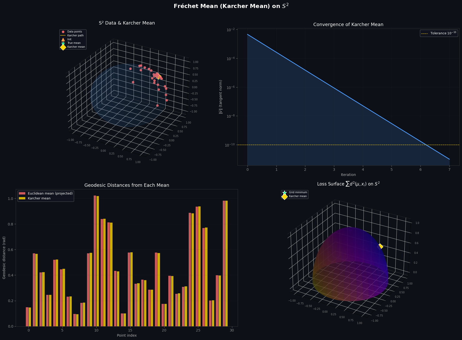
Figure saved.

Key Takeaways

  • The Fréchet mean generalises the Euclidean mean to curved spaces by replacing squared Euclidean distance with squared geodesic distance.
  • On $S^2$, the Karcher iteration converges in very few steps (typically < 20) for well-clustered data.
  • The naive approach of averaging Cartesian coordinates and projecting back onto the sphere is not the Fréchet mean in general — it minimises a different, Euclidean objective.
  • The same algorithmic skeleton works on any manifold for which you can implement $\exp$ and $\log$ — SO(3) rotations, symmetric positive-definite matrices, hyperbolic space, and beyond.