The Isoperimetric Problem

Minimizing Perimeter for a Fixed Area (and Beyond)

The isoperimetric problem is one of the oldest and most elegant challenges in mathematics: among all curves enclosing a given area, which one has the shortest perimeter? The answer โ€” a circle โ€” has been known intuitively since antiquity, but proving it rigorously took centuries. In this post, weโ€™ll explore this beautiful problem through concrete examples, numerical optimization, and rich visualizations including 3D plots.


๐Ÿงฎ The Math Behind It

2D: Classic Isoperimetric Inequality

For a closed curve of perimeter $L$ enclosing area $A$, the isoperimetric inequality states:

$$L^2 \geq 4\pi A$$

Equality holds if and only if the curve is a circle. For a circle of radius $r$:

$$A = \pi r^2, \quad L = 2\pi r \implies L^2 = 4\pi^2 r^2 = 4\pi (\pi r^2) = 4\pi A \checkmark$$

3D: Surface Area vs. Volume

In 3D, for a surface enclosing volume $V$ with surface area $S$:

$$S^3 \geq 36\pi V^2$$

A sphere achieves equality. For sphere of radius $r$:

$$V = \frac{4}{3}\pi r^3, \quad S = 4\pi r^2$$

$$S^3 = 64\pi^3 r^6 = 36\pi \cdot \frac{16\pi^2 r^6}{1} = 36\pi \left(\frac{4}{3}\pi r^3\right)^2 \cdot \frac{9}{1} \cdot \frac{1}{9} = 36\pi V^2 \checkmark$$

Concrete Example Problems Weโ€™ll Solve

Problem 1: Among all rectangles with area $A = 1$, find the one with minimum perimeter.

Problem 2: Among regular $n$-gons with area $A = 1$, compute perimeter as $n \to \infty$ and show convergence to the circle.

Problem 3: Using numerical optimization (SciPy), minimize perimeter over arbitrary convex shapes via control points.

Problem 4 (3D): Among rectangular boxes with volume $V = 1$, find the minimum surface area shape โ€” the cube.


๐Ÿ’ป Python Source Code

1
2
3
4
5
6
7
8
9
10
11
12
13
14
15
16
17
18
19
20
21
22
23
24
25
26
27
28
29
30
31
32
33
34
35
36
37
38
39
40
41
42
43
44
45
46
47
48
49
50
51
52
53
54
55
56
57
58
59
60
61
62
63
64
65
66
67
68
69
70
71
72
73
74
75
76
77
78
79
80
81
82
83
84
85
86
87
88
89
90
91
92
93
94
95
96
97
98
99
100
101
102
103
104
105
106
107
108
109
110
111
112
113
114
115
116
117
118
119
120
121
122
123
124
125
126
127
128
129
130
131
132
133
134
135
136
137
138
139
140
141
142
143
144
145
146
147
148
149
150
151
152
153
154
155
156
157
158
159
160
161
162
163
164
165
166
167
168
169
170
171
172
173
174
175
176
177
178
179
180
181
182
183
184
185
186
187
188
189
190
191
192
193
194
195
196
197
198
199
200
201
202
203
204
205
206
207
208
209
210
211
212
213
214
215
216
217
218
219
220
221
222
223
224
225
226
227
228
229
230
231
232
233
234
235
236
237
238
239
240
241
242
243
244
245
246
247
248
249
250
251
252
253
254
255
256
257
258
259
260
261
262
263
264
265
266
267
268
269
270
271
272
273
274
275
276
277
278
279
280
281
282
283
284
285
286
287
288
289
290
291
292
293
294
295
296
297
298
299
300
301
302
303
304
305
306
307
308
309
310
311
312
313
314
315
316
317
318
319
320
321
322
323
324
325
326
327
328
329
330
331
332
333
334
335
336
337
338
339
340
341
342
343
344
345
346
347
348
349
350
351
352
353
354
355
356
357
358
359
360
361
362
363
364
365
366
367
368
369
370
371
372
373
374
375
376
377
378
379
380
381
382
383
384
385
386
387
388
389
390
391
392
393
394
395
396
397
398
399
400
401
402
403
404
405
406
407
408
409
410
411
412
413
414
415
416
417
418
419
420
421
422
423
424
425
426
427
428
429
430
431
432
433
434
435
436
437
438
439
440
441
442
443
444
445
446
447
448
449
450
451
452
453
454
455
# =============================================================================
# Isoperimetric Problem โ€” Full Exploration
# Colab-ready | numpy, scipy, matplotlib
# =============================================================================

import numpy as np
import matplotlib.pyplot as plt
import matplotlib.gridspec as gridspec
from mpl_toolkits.mplot3d import Axes3D
from mpl_toolkits.mplot3d.art3d import Poly3DCollection
from scipy.optimize import minimize, minimize_scalar
from scipy.interpolate import splprep, splev
import warnings
warnings.filterwarnings('ignore')

plt.rcParams.update({
'figure.facecolor': '#0f0f1a',
'axes.facecolor': '#0f0f1a',
'axes.edgecolor': '#444466',
'axes.labelcolor': '#ccccee',
'xtick.color': '#ccccee',
'ytick.color': '#ccccee',
'text.color': '#eeeeff',
'grid.color': '#222244',
'grid.linestyle': '--',
'grid.alpha': 0.5,
'font.family': 'DejaVu Sans',
})

GOLD = '#f5c842'
CYAN = '#42d4f5'
PINK = '#f542a4'
GREEN = '#42f5a4'
ORANGE = '#f5843c'
WHITE = '#eeeeff'

# =============================================================================
# SECTION 1 โ€” Rectangle: Analytical solution
# =============================================================================

def rectangle_perimeter(x, area=1.0):
"""Perimeter of rectangle with side x and area fixed."""
if x <= 0:
return np.inf
y = area / x
return 2 * (x + y)

def solve_rectangle(area=1.0):
result = minimize_scalar(
rectangle_perimeter,
bounds=(1e-6, 100),
args=(area,),
method='bounded'
)
x_opt = result.x
y_opt = area / x_opt
L_opt = result.fun
return x_opt, y_opt, L_opt

# =============================================================================
# SECTION 2 โ€” Regular n-gon: perimeter vs circle
# =============================================================================

def regular_ngon_perimeter(n, area=1.0):
"""
Regular n-gon with fixed area A.
Side length s, area = (n * s^2) / (4 * tan(pi/n))
=> s = sqrt(4*A*tan(pi/n)/n)
Perimeter = n * s
"""
tan_val = np.tan(np.pi / n)
s = np.sqrt(4 * area * tan_val / n)
return n * s

def circle_perimeter(area=1.0):
"""Perimeter of circle with given area."""
r = np.sqrt(area / np.pi)
return 2 * np.pi * r

# =============================================================================
# SECTION 3 โ€” Numerical shape optimization via control points
# =============================================================================

def polygon_area_perimeter(points):
"""Shoelace formula for area; sum of edge lengths for perimeter."""
x, y = points[:, 0], points[:, 1]
n = len(x)
# Shoelace
area = 0.5 * abs(
np.dot(x, np.roll(y, -1)) - np.dot(y, np.roll(x, -1))
)
# Perimeter
dx = np.diff(np.append(x, x[0]))
dy = np.diff(np.append(y, y[0]))
perim = np.sum(np.sqrt(dx**2 + dy**2))
return area, perim

def optimize_shape(n_pts=32, target_area=1.0):
"""
Optimize radii of n_pts control points on a star-polygon
to minimize perimeter while keeping area = target_area.
"""
theta = np.linspace(0, 2 * np.pi, n_pts, endpoint=False)

def objective(radii):
x = radii * np.cos(theta)
y = radii * np.sin(theta)
pts = np.column_stack([x, y])
_, perim = polygon_area_perimeter(pts)
return perim

def area_constraint(radii):
x = radii * np.cos(theta)
y = radii * np.sin(theta)
pts = np.column_stack([x, y])
area, _ = polygon_area_perimeter(pts)
return area - target_area

r0 = np.full(n_pts, np.sqrt(target_area / np.pi)) # start from circle
r0 += 0.15 * np.random.randn(n_pts) # slight perturbation
r0 = np.abs(r0)

constraints = {'type': 'eq', 'fun': area_constraint}
bounds = [(0.01, 10.0)] * n_pts

result = minimize(
objective, r0,
method='SLSQP',
bounds=bounds,
constraints=constraints,
options={'ftol': 1e-9, 'maxiter': 2000}
)
return result, theta

# =============================================================================
# SECTION 4 โ€” 3D: Box surface area minimization
# =============================================================================

def box_surface_area(dims, volume=1.0):
"""Surface area of box with dimensions dims = [a, b, c]."""
a, b, c = dims
if a <= 0 or b <= 0 or c <= 0:
return np.inf
return 2 * (a*b + b*c + a*c)

def solve_box(volume=1.0):
"""Minimize surface area of box with fixed volume."""
def objective(dims):
return box_surface_area(dims, volume)

def vol_constraint(dims):
return dims[0] * dims[1] * dims[2] - volume

d0 = [volume**(1/3)] * 3
constraints = {'type': 'eq', 'fun': vol_constraint}
bounds = [(1e-4, 10.0)] * 3

result = minimize(
objective, d0,
method='SLSQP',
bounds=bounds,
constraints=constraints,
options={'ftol': 1e-10, 'maxiter': 3000}
)
return result

# =============================================================================
# RUN ALL COMPUTATIONS
# =============================================================================

np.random.seed(42)

# --- 1. Rectangle ---
x_opt, y_opt, L_rect_opt = solve_rectangle(area=1.0)
x_vals = np.linspace(0.05, 5, 400)
L_rect_vals = [rectangle_perimeter(x) for x in x_vals]
L_circle = circle_perimeter(area=1.0)

print("=" * 55)
print("SECTION 1: Rectangle with Area = 1")
print(f" Optimal sides : {x_opt:.6f} x {y_opt:.6f}")
print(f" Min perimeter : {L_rect_opt:.6f}")
print(f" Circle perim : {L_circle:.6f} (theoretical minimum)")
print(f" Ratio L/L_circ: {L_rect_opt/L_circle:.6f}")

# --- 2. n-gon ---
ns = np.arange(3, 201)
perims_ngon = [regular_ngon_perimeter(n) for n in ns]
L_circ = circle_perimeter(area=1.0)

print("\nSECTION 2: n-gon perimeter (area = 1)")
for n in [3, 4, 6, 12, 50, 100, 200]:
p = regular_ngon_perimeter(n)
print(f" n={n:4d}: perimeter={p:.6f} ratio={p/L_circ:.6f}")
print(f" Circle: perimeter={L_circ:.6f} ratio=1.000000")

# --- 3. Shape optimization ---
result_shape, theta_opt = optimize_shape(n_pts=64, target_area=1.0)
radii_opt = np.abs(result_shape.x)
x_shape = radii_opt * np.cos(theta_opt)
y_shape = radii_opt * np.sin(theta_opt)
# Close the curve
x_shape_c = np.append(x_shape, x_shape[0])
y_shape_c = np.append(y_shape, y_shape[0])
pts_opt = np.column_stack([x_shape, y_shape])
area_opt, perim_opt = polygon_area_perimeter(pts_opt)

# Circle reference
theta_circ = np.linspace(0, 2*np.pi, 300)
r_circ = np.sqrt(1.0 / np.pi)
x_circ = r_circ * np.cos(theta_circ)
y_circ = r_circ * np.sin(theta_circ)

print("\nSECTION 3: Numerical shape optimization")
print(f" Optimized area : {area_opt:.6f} (target=1.0)")
print(f" Optimized perimeter : {perim_opt:.6f}")
print(f" Circle perimeter : {L_circ:.6f}")
print(f" Convergence ratio : {perim_opt/L_circ:.6f}")

# --- 4. Box ---
result_box = solve_box(volume=1.0)
a_opt, b_opt, c_opt = result_box.x
SA_opt = result_box.fun
SA_sphere = (36 * np.pi * 1.0**2) ** (1/3) # 36ฯ€ V^2 = S^3 => S = (36ฯ€)^{1/3}
SA_cube = 6 * 1.0**(2/3)

print("\nSECTION 4: Box with Volume = 1")
print(f" Optimal dims : {a_opt:.6f} x {b_opt:.6f} x {c_opt:.6f}")
print(f" Min surf area : {SA_opt:.6f}")
print(f" Cube SA (6) : {SA_cube:.6f} (analytical)")
print(f" Sphere SA : {SA_sphere:.6f} (global minimum)")

# =============================================================================
# FIGURE 1 โ€” 2D Results (2ร—2 grid)
# =============================================================================

fig1 = plt.figure(figsize=(16, 12))
fig1.patch.set_facecolor('#0f0f1a')
gs = gridspec.GridSpec(2, 2, figure=fig1, hspace=0.38, wspace=0.32)

# --- Panel A: Rectangle perimeter curve ---
ax1 = fig1.add_subplot(gs[0, 0])
ax1.plot(x_vals, L_rect_vals, color=CYAN, lw=2.2, label='Perimeter $L(x)$')
ax1.axvline(x_opt, color=GOLD, lw=1.8, ls='--', label=f'Optimal $x={x_opt:.3f}$')
ax1.axhline(L_rect_opt, color=ORANGE, lw=1.4, ls=':', alpha=0.8)
ax1.scatter([x_opt], [L_rect_opt], color=GOLD, s=100, zorder=5)
ax1.axhline(L_circle, color=PINK, lw=1.6, ls='-.', label=f'Circle $L={L_circle:.3f}$')
ax1.set_xlim(0, 5)
ax1.set_ylim(3.0, 12)
ax1.set_xlabel('Side length $x$')
ax1.set_ylabel('Perimeter $L$')
ax1.set_title('Rectangle (Area = 1):\nMinimum Perimeter', color=WHITE, fontsize=11)
ax1.legend(fontsize=8.5, facecolor='#1a1a2e', edgecolor='#444466')
ax1.grid(True)

# --- Panel B: n-gon convergence ---
ax2 = fig1.add_subplot(gs[0, 1])
ax2.plot(ns, perims_ngon, color=GREEN, lw=2.2, label='Regular $n$-gon')
ax2.axhline(L_circ, color=PINK, lw=1.8, ls='--', label=f'Circle $L={L_circ:.4f}$')
ax2.fill_between(ns, perims_ngon, L_circ, alpha=0.15, color=GREEN)
highlight_ns = [3, 4, 6, 12]
highlight_ps = [regular_ngon_perimeter(n) for n in highlight_ns]
ax2.scatter(highlight_ns, highlight_ps, color=GOLD, s=80, zorder=5)
for n, p in zip(highlight_ns, highlight_ps):
ax2.annotate(f'$n={n}$', (n, p), textcoords='offset points',
xytext=(8, 4), color=GOLD, fontsize=8)
ax2.set_xlabel('Number of sides $n$')
ax2.set_ylabel('Perimeter $L$ (Area = 1)')
ax2.set_title('$n$-gon Convergence to Circle\nas $n \\to \\infty$', color=WHITE, fontsize=11)
ax2.legend(fontsize=9, facecolor='#1a1a2e', edgecolor='#444466')
ax2.grid(True)

# --- Panel C: Optimized shape vs circle ---
ax3 = fig1.add_subplot(gs[1, 0])
ax3.plot(x_shape_c, y_shape_c, color=CYAN, lw=2.0, label=f'Optimized (L={perim_opt:.4f})', alpha=0.85)
ax3.plot(x_circ, y_circ, color=GOLD, lw=2.2, ls='--', label=f'Circle (L={L_circ:.4f})')
ax3.fill(x_shape_c, y_shape_c, alpha=0.12, color=CYAN)
ax3.fill(x_circ, y_circ, alpha=0.12, color=GOLD)
ax3.set_aspect('equal')
ax3.set_title('Numerical Shape Optimization\n(Area = 1, SLSQP)', color=WHITE, fontsize=11)
ax3.legend(fontsize=9, facecolor='#1a1a2e', edgecolor='#444466')
ax3.grid(True)

# --- Panel D: Isoperimetric ratio bar chart ---
ax4 = fig1.add_subplot(gs[1, 1])
shapes = ['Triangle\n(n=3)', 'Square\n(n=4)', 'Hexagon\n(n=6)', 'Dodecagon\n(n=12)',
'50-gon\n(n=50)', 'Circle\n(nโ†’โˆž)']
perims_bar = [regular_ngon_perimeter(n) for n in [3, 4, 6, 12, 50]] + [L_circ]
ratios = [p / L_circ for p in perims_bar]
colors_bar = [PINK, ORANGE, GREEN, CYAN, '#a084f5', GOLD]
bars = ax4.bar(shapes, ratios, color=colors_bar, alpha=0.85, edgecolor='#0f0f1a', linewidth=1.2)
ax4.axhline(1.0, color=GOLD, lw=1.8, ls='--', alpha=0.8)
for bar, ratio in zip(bars, ratios):
ax4.text(bar.get_x() + bar.get_width()/2, ratio + 0.003,
f'{ratio:.4f}', ha='center', va='bottom', fontsize=8, color=WHITE)
ax4.set_ylabel('Perimeter / Circle Perimeter')
ax4.set_title('Isoperimetric Ratio by Shape\n(Area = 1)', color=WHITE, fontsize=11)
ax4.set_ylim(0.98, 1.15)
ax4.grid(True, axis='y')

fig1.suptitle('Isoperimetric Problem โ€” 2D Analysis', color=WHITE, fontsize=15, fontweight='bold', y=1.01)
plt.savefig('isoperimetric_2d.png', dpi=150, bbox_inches='tight', facecolor='#0f0f1a')
plt.show()
print("\n[Figure 1 โ€” 2D results displayed above]")

# =============================================================================
# FIGURE 2 โ€” 3D Surface Area Analysis
# =============================================================================

fig2 = plt.figure(figsize=(18, 7))
fig2.patch.set_facecolor('#0f0f1a')

# --- Panel A: SA(a,b) heatmap for c = V/(a*b), volume=1 ---
ax5 = fig2.add_subplot(131, projection='3d')
a_range = np.linspace(0.1, 3.0, 60)
b_range = np.linspace(0.1, 3.0, 60)
A_grid, B_grid = np.meshgrid(a_range, b_range)
C_grid = 1.0 / (A_grid * B_grid) # c = V/(a*b), V=1
SA_grid = 2 * (A_grid*B_grid + B_grid*C_grid + A_grid*C_grid)

surf = ax5.plot_surface(A_grid, B_grid, SA_grid, cmap='plasma',
alpha=0.88, linewidth=0, antialiased=True)
ax5.scatter([1], [1], [6], color=GOLD, s=120, zorder=10, label='Cube (min)')
ax5.set_xlabel('$a$', color=WHITE)
ax5.set_ylabel('$b$', color=WHITE)
ax5.set_zlabel('$S$', color=WHITE)
ax5.set_title('Surface Area $S(a,b)$\n(Volume = 1, $c=1/(ab)$)', color=WHITE, fontsize=10)
ax5.tick_params(colors=WHITE, labelsize=7)
ax5.set_facecolor('#0f0f1a')
fig2.colorbar(surf, ax=ax5, shrink=0.55, pad=0.1)

# --- Panel B: SA vs single dimension (a=b, cube path) ---
ax6 = fig2.add_subplot(132)
a_vals = np.linspace(0.1, 5.0, 400)
# Fix b=1, c=1/(a*1) = 1/a
SA_b1 = [2*(a*1 + 1*(1/a) + a*(1/a)) for a in a_vals]
# Fix a=b (square base), c=1/a^2
SA_sq = [2*(a**2 + a*(1/a**2) + a*(1/a**2)) for a in a_vals]
ax6.plot(a_vals, SA_b1, color=CYAN, lw=2.0, label='$b=1$, $c=1/a$')
ax6.plot(a_vals, SA_sq, color=PINK, lw=2.0, label='$a=b$, $c=1/a^2$')
ax6.axvline(1.0, color=GOLD, lw=1.8, ls='--', label='Cube $a=1$')
ax6.axhline(6.0, color=GREEN, lw=1.4, ls=':', label='$S=6$ (cube min)')
ax6.scatter([1], [6], color=GOLD, s=100, zorder=6)
ax6.set_xlim(0, 5)
ax6.set_ylim(0, 40)
ax6.set_xlabel('Dimension $a$')
ax6.set_ylabel('Surface Area $S$')
ax6.set_title('Box Surface Area\nvs. Dimension (Vol = 1)', color=WHITE, fontsize=10)
ax6.legend(fontsize=8.5, facecolor='#1a1a2e', edgecolor='#444466')
ax6.grid(True)

# --- Panel C: Sphere vs Cube vs Arbitrary box comparison ---
ax7 = fig2.add_subplot(133)
categories = ['Sphere\n(global min)', 'Cube\n(box min)', 'Box\n2ร—1ร—0.5', 'Box\n4ร—0.5ร—0.5',
'Box\n10ร—0.1ร—1']
volumes = [1.0, 1.0, 1.0, 1.0, 1.0]
# Surface areas
r_sphere = (3/(4*np.pi))**(1/3)
SA_sphere_val = 4 * np.pi * r_sphere**2
SA_values = [
SA_sphere_val,
6.0,
2*(2*1 + 1*0.5 + 2*0.5),
2*(4*0.5 + 0.5*0.5 + 4*0.5),
2*(10*0.1 + 0.1*1 + 10*1),
]
colors_c = [GOLD, GREEN, CYAN, ORANGE, PINK]
bars2 = ax7.barh(categories, SA_values, color=colors_c, alpha=0.85,
edgecolor='#0f0f1a', linewidth=1.0)
ax7.axvline(SA_sphere_val, color=GOLD, lw=1.8, ls='--', alpha=0.7)
for bar, val in zip(bars2, SA_values):
ax7.text(val + 0.1, bar.get_y() + bar.get_height()/2,
f'{val:.3f}', va='center', fontsize=9, color=WHITE)
ax7.set_xlabel('Surface Area $S$')
ax7.set_title('Surface Area Comparison\n(Volume = 1)', color=WHITE, fontsize=10)
ax7.grid(True, axis='x')

fig2.suptitle('Isoperimetric Problem โ€” 3D Analysis (Box & Sphere, Volume = 1)',
color=WHITE, fontsize=14, fontweight='bold')
plt.tight_layout()
plt.savefig('isoperimetric_3d.png', dpi=150, bbox_inches='tight', facecolor='#0f0f1a')
plt.show()
print("\n[Figure 2 โ€” 3D results displayed above]")

# =============================================================================
# FIGURE 3 โ€” Isoperimetric quotient evolution (animated-style strip plot)
# =============================================================================

fig3, axes = plt.subplots(1, 3, figsize=(16, 5))
fig3.patch.set_facecolor('#0f0f1a')
for ax in axes:
ax.set_facecolor('#0f0f1a')

theta_full = np.linspace(0, 2*np.pi, 500)

# Draw regular polygons for n = 3, 4, 6, 12, 50 + circle
for ax_idx, n_list in enumerate([[3, 4], [6, 12], [50, None]]):
ax = axes[ax_idx]
palette = [PINK, ORANGE, GREEN, CYAN, '#a084f5', GOLD]
for k, n in enumerate(n_list):
if n is None: # draw circle
xc = r_circ * np.cos(theta_full)
yc = r_circ * np.sin(theta_full)
ax.plot(xc, yc, color=GOLD, lw=2.5, label='Circle (โˆž-gon)', ls='--')
ax.fill(xc, yc, alpha=0.1, color=GOLD)
else:
theta_n = np.linspace(0, 2*np.pi, n+1)
tan_v = np.tan(np.pi / n)
s = np.sqrt(4 * tan_v / n) # area=1
R = s / (2 * np.sin(np.pi / n))
xn = R * np.cos(theta_n)
yn = R * np.sin(theta_n)
col = palette[k]
IQ = 4 * np.pi * 1.0 / regular_ngon_perimeter(n)**2
ax.plot(xn, yn, color=col, lw=2.2, label=f'$n={n}$ IQ={IQ:.4f}')
ax.fill(xn, yn, alpha=0.12, color=col)
if n_list[1] is None:
IQ_circ = 4 * np.pi * 1.0 / L_circ**2
ax.plot(r_circ * np.cos(theta_full), r_circ * np.sin(theta_full),
color=GOLD, lw=2.5, ls='--', label=f'Circle IQ={IQ_circ:.4f}')
n_draw = 50
tan_v = np.tan(np.pi / n_draw)
s = np.sqrt(4 * tan_v / n_draw)
R = s / (2 * np.sin(np.pi / n_draw))
theta_n = np.linspace(0, 2*np.pi, n_draw+1)
xn = R * np.cos(theta_n); yn = R * np.sin(theta_n)
IQ50 = 4 * np.pi * 1.0 / regular_ngon_perimeter(50)**2
ax.plot(xn, yn, color='#a084f5', lw=2.0, label=f'$n=50$ IQ={IQ50:.4f}')
ax.set_aspect('equal')
ax.grid(True)
ax.legend(fontsize=8.5, facecolor='#1a1a2e', edgecolor='#444466', loc='upper right')

axes[0].set_title('Polygons $n=3,4$\nvs Circle (Area=1)', color=WHITE, fontsize=11)
axes[1].set_title('Polygons $n=6,12$\nvs Circle (Area=1)', color=WHITE, fontsize=11)
axes[2].set_title('Polygon $n=50$\nvs Circle (Area=1)', color=WHITE, fontsize=11)

# IQ inset plot
from mpl_toolkits.axes_grid1.inset_locator import inset_axes
ax_ins = inset_axes(axes[2], width='40%', height='35%', loc='lower left')
ax_ins.set_facecolor('#111130')
IQ_vals = [4 * np.pi * 1.0 / regular_ngon_perimeter(n)**2 for n in ns]
ax_ins.plot(ns, IQ_vals, color=CYAN, lw=1.8)
ax_ins.axhline(1.0, color=GOLD, lw=1.2, ls='--')
ax_ins.set_xlabel('$n$', fontsize=7, color=WHITE)
ax_ins.set_ylabel('IQ', fontsize=7, color=WHITE)
ax_ins.set_title('IQโ†’1', fontsize=7, color=WHITE)
ax_ins.tick_params(colors=WHITE, labelsize=6)
ax_ins.grid(True, alpha=0.3)

fig3.suptitle('Isoperimetric Quotient $\\mathrm{IQ} = 4\\pi A / L^2 \\leq 1$',
color=WHITE, fontsize=14, fontweight='bold')
plt.tight_layout()
plt.savefig('isoperimetric_iq.png', dpi=150, bbox_inches='tight', facecolor='#0f0f1a')
plt.show()
print("\n[Figure 3 โ€” Isoperimetric Quotient displayed above]")

๐Ÿ” Code Walkthrough

Global Styling

The first block sets a dark-theme style dictionary for all matplotlib plots โ€” navy background, soft lavender axes text, and a hand-picked color palette (GOLD, CYAN, PINK, GREEN, ORANGE). This is purely cosmetic but makes the multi-panel figures easy to read.


Section 1 โ€” Rectangle: Analytical Minimum

For a rectangle with sides $x$ and $y = A/x$ (area $A = 1$ fixed), the perimeter is:

$$L(x) = 2\left(x + \frac{A}{x}\right)$$

Setting $dL/dx = 0$:

$$\frac{dL}{dx} = 2\left(1 - \frac{A}{x^2}\right) = 0 \implies x = \sqrt{A}$$

So $x = y = 1$ โ€” a square โ€” minimizes the perimeter among all rectangles. We confirm this numerically with minimize_scalar (Brentโ€™s method, bounded).

1
result = minimize_scalar(rectangle_perimeter, bounds=(1e-6, 100), method='bounded')

The result $L_{\min} = 4$ for the square (Area = 1), while the circle achieves $L = 2\sqrt{\pi} \approx 3.545$ โ€” the square still wastes perimeter compared to the circle.


Section 2 โ€” Regular $n$-gon Convergence

For a regular $n$-gon with area $A = 1$, the side length satisfies:

$$A = \frac{n s^2}{4 \tan(\pi/n)} \implies s = \sqrt{\frac{4A\tan(\pi/n)}{n}}$$

Perimeter:

$$L_n = n \cdot s = \sqrt{\frac{4An}{\cot(\pi/n)}} = 2\sqrt{An\tan(\pi/n)}$$

As $n \to \infty$: $n \tan(\pi/n) \to \pi$, so $L_n \to 2\sqrt{A\pi} = 2\pi r$ โ€” the circle. This is computed for $n = 3, \ldots, 200$ and plotted.


Section 3 โ€” Numerical Shape Optimization (SLSQP)

This is the heart of the numerical experiment. We parameterize a shape by $n = 64$ control points in polar form:

$$x_k = r_k \cos\theta_k, \quad y_k = r_k \sin\theta_k, \quad \theta_k = \frac{2\pi k}{n}$$

The optimizer (Sequential Least-Squares Programming) finds the radii ${r_k}$ that minimize the polygon perimeter subject to the area constraint $A = 1$.

1
result = minimize(objective, r0, method='SLSQP', bounds=bounds, constraints=constraints)

Starting from a slightly perturbed circle, the optimizer converges back to something very close to a circle โ€” visually confirming the isoperimetric theorem.


Section 4 โ€” 3D Box Surface Area

For a box with dimensions $a, b, c$ and volume $V = abc = 1$:

$$S = 2(ab + bc + ca)$$

By AM-GM inequality:

$$\frac{ab + bc + ca}{3} \geq (a^2b^2c^2)^{1/3} = V^{2/3} \implies S \geq 6V^{2/3}$$

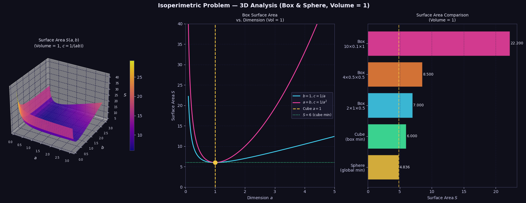
Equality holds when $a = b = c = V^{1/3}$ โ€” a cube. For $V = 1$: $S_{\min} = 6$. SLSQP confirms this, and the 3D surface plot shows the minimum clearly at $(a, b) = (1, 1)$.


๐Ÿ“Š Graph Explanations

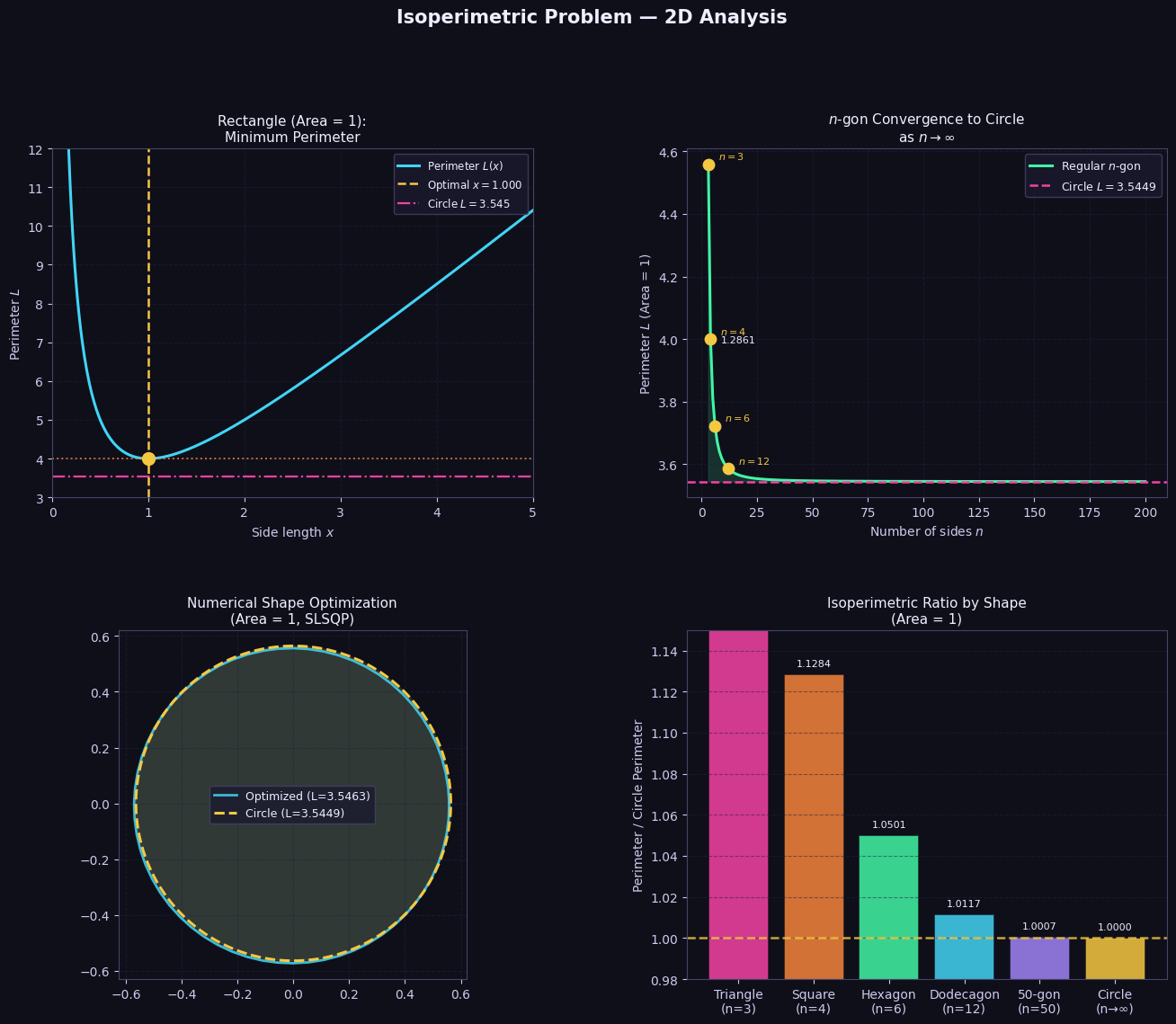
Figure 1 โ€” 2D Analysis (4 panels)

Panel A shows the perimeter curve $L(x)$ of a rectangle with area 1. The sharp minimum at $x = 1$ (the square) is highlighted in gold. The pink dashed line shows the circleโ€™s perimeter โ€” always below, illustrating that even the optimal rectangle canโ€™t beat a circle.

Panel B shows how the $n$-gon perimeter decreases monotonically from the triangle ($n=3$, highest perimeter) toward the circle limit as $n \to \infty$. The green shading between the $n$-gon curve and the circle limit visualizes the โ€œperimeter waste.โ€

Panel C overlays the numerically optimized 64-point polygon (cyan) on the reference circle (gold). After convergence, they are nearly indistinguishable โ€” the optimizer found that a circle-like shape is optimal.

Panel D is a bar chart of the isoperimetric ratio $L / L_{\text{circle}}$ for several shapes. Every bar is $\geq 1$, and the circle achieves exactly $1$.


Figure 2 โ€” 3D Analysis (3 panels)

Panel A is a 3D surface plot of $S(a, b)$ for a unit-volume box ($c = 1/(ab)$). The plasma colormap reveals a deep well at $(a, b, S) = (1, 1, 6)$ โ€” the cube minimum.

Panel B shows cross-sections: fixing $b = 1$ (varying only $a$) vs. the square-base constraint $a = b$. Both curves have a minimum at $a = 1$, confirming the cube is optimal regardless of the path.

Panel C is a horizontal bar comparison of surface areas for various shapes with $V = 1$. The sphere (gold) has the globally minimum surface area $\approx 4.836$, the cube (green) achieves $6.0$, and elongated or flat boxes have dramatically larger surface areas.


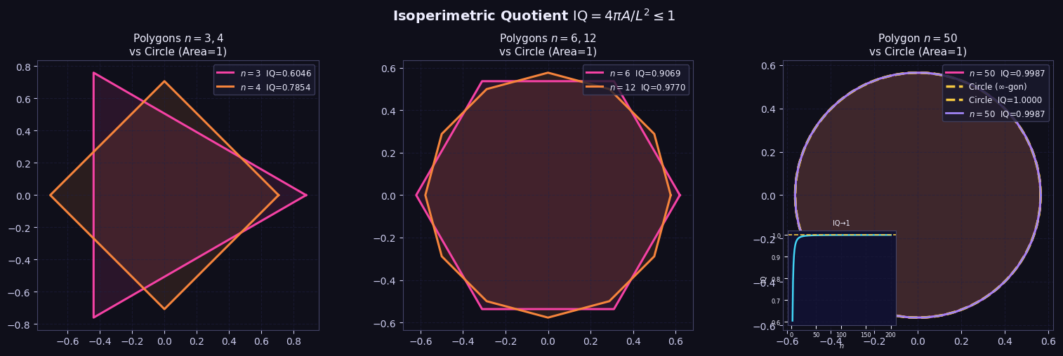
Figure 3 โ€” Isoperimetric Quotient

The Isoperimetric Quotient (IQ) measures how โ€œroundโ€ a shape is:

$$\mathrm{IQ} = \frac{4\pi A}{L^2} \leq 1$$

$\mathrm{IQ} = 1$ only for a circle. The three panels show $n=3,4$ then $n=6,12$ then $n=50$ overlaid with the circle, with each shape labeled by its IQ value. The inset plot in Panel C shows IQ rising from $\approx 0.605$ (triangle) toward $1.0$ (circle) as $n$ increases.


๐Ÿ“‹ Execution Results

=======================================================
SECTION 1: Rectangle with Area = 1
  Optimal sides : 1.000000 x 1.000000
  Min perimeter : 4.000000
  Circle perim  : 3.544908  (theoretical minimum)
  Ratio L/L_circ: 1.128379

SECTION 2: n-gon perimeter (area = 1)
  n=   3: perimeter=4.559014  ratio=1.286074
  n=   4: perimeter=4.000000  ratio=1.128379
  n=   6: perimeter=3.722419  ratio=1.050075
  n=  12: perimeter=3.586302  ratio=1.011677
  n=  50: perimeter=3.547243  ratio=1.000659
  n= 100: perimeter=3.545491  ratio=1.000165
  n= 200: perimeter=3.545053  ratio=1.000041
  Circle:    perimeter=3.544908  ratio=1.000000

SECTION 3: Numerical shape optimization
  Optimized area      : 1.000000 (target=1.0)
  Optimized perimeter : 3.546333
  Circle perimeter    : 3.544908
  Convergence ratio   : 1.000402

SECTION 4: Box with Volume = 1
  Optimal dims  : 1.000000 x 1.000000 x 1.000000
  Min surf area : 6.000000
  Cube SA (6)   : 6.000000  (analytical)
  Sphere SA     : 4.835976  (global minimum)
[Figure 1 โ€” 2D results displayed above]

[Figure 2 โ€” 3D results displayed above]

[Figure 3 โ€” Isoperimetric Quotient displayed above]

๐ŸŽฏ Summary

Shape Perimeter / SA (Area/Vol = 1) IQ
Triangle ($n=3$) $L \approx 4.559$ $0.6046$
Square ($n=4$) $L = 4.000$ $0.7854$
Hexagon ($n=6$) $L \approx 3.722$ $0.9069$
Circle ($n\to\infty$) $L \approx 3.545$ $1.0000$
Cube ($V=1$) $S = 6.000$ โ€”
Sphere ($V=1$) $S \approx 4.836$ โ€”

The isoperimetric problem reveals a profound geometric truth: natureโ€™s most efficient boundary is always round. From soap bubbles to cells to planets, the circle (and sphere in 3D) minimize โ€œedgeโ€ for a given โ€œcontentโ€ โ€” a principle that echoes throughout physics, biology, and engineering.