Integrated Optimization of Credit Risk and Fraud Risk

A Unified Framework

Managing a lending portfolio means fighting a war on two fronts simultaneously. On one side, credit risk — the danger that a borrower simply can’t repay. On the other, fraud risk — the danger that a borrower never intended to repay. Optimizing for one while ignoring the other leads to portfolios that look clean on paper but bleed money in practice.

This post walks through a concrete, mathematically grounded model that jointly optimizes both risks, solves it in Python, and visualizes the results in 2D and 3D.


The Problem Setup

Imagine a bank evaluating 1,000 loan applicants. Each applicant has two scores:

  • $s_c \in [0, 1]$ — credit score (higher = less likely to default)
  • $s_f \in [0, 1]$ — fraud score (higher = less likely to be fraudulent)

The bank must set two thresholds:

  • $\tau_c$ — minimum credit score to approve
  • $\tau_f$ — minimum fraud score to approve

An applicant is approved if and only if $s_c \geq \tau_c$ and $s_f \geq \tau_f$.


The Mathematical Model

Expected profit for an approved applicant:

$$\Pi(s_c, s_f) = R \cdot (1 - P_d(s_c)) \cdot (1 - P_f(s_f)) - L_d \cdot P_d(s_c) - L_f \cdot P_f(s_f)$$

Where:

  • $R$ = revenue from a performing loan
  • $L_d$ = loss given credit default
  • $L_f$ = loss given fraud
  • $P_d(s_c) = e^{-\alpha s_c}$ — default probability (decreasing in credit score)
  • $P_f(s_f) = e^{-\beta s_f}$ — fraud probability (decreasing in fraud score)

Total expected profit over all applicants:

$$\mathcal{J}(\tau_c, \tau_f) = \sum_{i=1}^{N} \mathbf{1}[s_c^{(i)} \geq \tau_c,\ s_f^{(i)} \geq \tau_f] \cdot \Pi(s_c^{(i)}, s_f^{(i)})$$

Optimization problem:

$$\max_{\tau_c,\ \tau_f \in [0,1]} \quad \mathcal{J}(\tau_c, \tau_f)$$

subject to:

$$\text{Approval Rate} \geq \delta_{\min}$$

$$\mathbb{E}[P_d \mid \text{approved}] \leq \rho_c$$

$$\mathbb{E}[P_f \mid \text{approved}] \leq \rho_f$$


The Integrated Risk Score

Rather than treating the two risks independently, we define a combined risk score:

$$\mathcal{R}(s_c, s_f) = \lambda \cdot P_d(s_c) + (1 - \lambda) \cdot P_f(s_f), \quad \lambda \in [0,1]$$

The parameter $\lambda$ controls the trade-off weight between credit and fraud risk. The bank can then set a single threshold $\tau_r$ on $\mathcal{R}$, or jointly optimize $(\tau_c, \tau_f)$ on the full profit surface.


Python Implementation

1
2
3
4
5
6
7
8
9
10
11
12
13
14
15
16
17
18
19
20
21
22
23
24
25
26
27
28
29
30
31
32
33
34
35
36
37
38
39
40
41
42
43
44
45
46
47
48
49
50
51
52
53
54
55
56
57
58
59
60
61
62
63
64
65
66
67
68
69
70
71
72
73
74
75
76
77
78
79
80
81
82
83
84
85
86
87
88
89
90
91
92
93
94
95
96
97
98
99
100
101
102
103
104
105
106
107
108
109
110
111
112
113
114
115
116
117
118
119
120
121
122
123
124
125
126
127
128
129
130
131
132
133
134
135
136
137
138
139
140
141
142
143
144
145
146
147
148
149
150
151
152
153
154
155
156
157
158
159
160
161
162
163
164
165
166
167
168
169
170
171
172
173
174
175
176
177
178
179
180
181
182
183
184
185
186
187
188
189
190
191
192
193
194
195
196
197
198
199
200
201
202
203
204
205
206
207
208
209
210
211
212
213
214
215
216
217
218
219
220
221
222
223
224
225
226
227
228
229
230
231
232
233
234
235
236
237
238
239
240
241
242
243
244
245
246
247
248
249
250
251
252
253
254
255
256
257
258
259
260
261
262
263
264
265
266
267
268
269
270
271
272
273
274
275
276
277
278
279
280
281
282
283
284
285
286
287
288
289
290
291
292
293
294
295
296
297
298
299
300
301
302
303
304
305
306
307
308
309
310
311
312
313
314
315
316
317
318
319
320
321
322
323
324
325
326
327
328
329
330
331
332
333
334
335
336
337
338
339
340
341
342
343
344
345
346
347
348
# ============================================================
# Integrated Credit Risk & Fraud Risk Optimization
# ============================================================

import numpy as np
import pandas as pd
import matplotlib.pyplot as plt
import matplotlib.gridspec as gridspec
from matplotlib import cm
from scipy.optimize import differential_evolution
from mpl_toolkits.mplot3d import Axes3D
import warnings
warnings.filterwarnings('ignore')

# ── Reproducibility ──────────────────────────────────────────
np.random.seed(42)

# ============================================================
# 1. SIMULATION: Generate Synthetic Applicant Population
# ============================================================
N = 1000 # number of applicants

# Credit scores and fraud scores are correlated (rho = 0.3)
# because good borrowers tend to be less fraudulent too
mean = [0.5, 0.5]
cov = [[0.04, 0.012],
[0.012, 0.04]]
scores = np.random.multivariate_normal(mean, cov, N)
credit_scores = np.clip(scores[:, 0], 0.01, 0.99)
fraud_scores = np.clip(scores[:, 1], 0.01, 0.99)

# ============================================================
# 2. BUSINESS PARAMETERS
# ============================================================
R = 5000 # revenue if loan performs ($)
L_d = 15000 # loss given credit default ($)
L_f = 20000 # loss given fraud ($)

alpha = 4.0 # sensitivity of default prob to credit score
beta = 5.0 # sensitivity of fraud prob to fraud score

# Constraint parameters
delta_min = 0.20 # at least 20% approval rate
rho_c = 0.15 # max average default probability among approved
rho_f = 0.10 # max average fraud probability among approved

# ============================================================
# 3. CORE PROBABILITY & PROFIT FUNCTIONS
# ============================================================
def prob_default(sc, alpha=alpha):
"""P_d(s_c) = exp(-alpha * s_c)"""
return np.exp(-alpha * sc)

def prob_fraud(sf, beta=beta):
"""P_f(s_f) = exp(-beta * s_f)"""
return np.exp(-beta * sf)

def expected_profit_per_applicant(sc, sf):
"""
Pi(s_c, s_f) = R*(1-P_d)*(1-P_f) - L_d*P_d - L_f*P_f
"""
pd_ = prob_default(sc)
pf_ = prob_fraud(sf)
return R * (1 - pd_) * (1 - pf_) - L_d * pd_ - L_f * pf_

# Pre-compute profits for all applicants
all_profits = expected_profit_per_applicant(credit_scores, fraud_scores)
all_pd = prob_default(credit_scores)
all_pf = prob_fraud(fraud_scores)

# ============================================================
# 4. OBJECTIVE FUNCTION (to MAXIMIZE)
# ============================================================
def total_profit(tau_c, tau_f, return_stats=False):
"""
Compute total expected profit for given thresholds.
Returns a large negative number if constraints are violated.
"""
mask = (credit_scores >= tau_c) & (fraud_scores >= tau_f)
n_approved = mask.sum()

if n_approved == 0:
if return_stats:
return -1e9, 0, 0, 0, 0
return -1e9

approval_rate = n_approved / N
avg_pd = all_pd[mask].mean()
avg_pf = all_pf[mask].mean()
profit = all_profits[mask].sum()

# Constraint penalties
if approval_rate < delta_min:
profit -= 1e8 * (delta_min - approval_rate)
if avg_pd > rho_c:
profit -= 1e8 * (avg_pd - rho_c)
if avg_pf > rho_f:
profit -= 1e8 * (avg_pf - rho_f)

if return_stats:
return profit, approval_rate, avg_pd, avg_pf, n_approved
return profit

# ============================================================
# 5. GRID SEARCH — Build the Full Profit Surface
# ============================================================
grid_size = 80
tau_c_vals = np.linspace(0.01, 0.99, grid_size)
tau_f_vals = np.linspace(0.01, 0.99, grid_size)
TC, TF = np.meshgrid(tau_c_vals, tau_f_vals)

# Vectorized grid search
profit_surface = np.zeros((grid_size, grid_size))
for i, tc in enumerate(tau_c_vals):
for j, tf in enumerate(tau_f_vals):
profit_surface[j, i] = total_profit(tc, tf)

# Replace penalty values with NaN for plotting
profit_display = profit_surface.copy()
profit_display[profit_surface < -1e6] = np.nan

# ============================================================
# 6. GLOBAL OPTIMIZATION via Differential Evolution
# ============================================================
def neg_profit(params):
return -total_profit(params[0], params[1])

bounds = [(0.01, 0.99), (0.01, 0.99)]
result = differential_evolution(
neg_profit,
bounds,
seed=42,
maxiter=500,
tol=1e-8,
popsize=15,
mutation=(0.5, 1.5),
recombination=0.9
)

tau_c_opt, tau_f_opt = result.x
profit_opt, ar_opt, pd_opt, pf_opt, n_opt = total_profit(
tau_c_opt, tau_f_opt, return_stats=True
)

print("=" * 55)
print(" OPTIMIZATION RESULTS")
print("=" * 55)
print(f" Optimal credit threshold τ_c : {tau_c_opt:.4f}")
print(f" Optimal fraud threshold τ_f : {tau_f_opt:.4f}")
print(f" Total expected profit : ${profit_opt:,.0f}")
print(f" Applicants approved : {n_opt} / {N}")
print(f" Approval rate : {ar_opt:.1%}")
print(f" Avg default probability : {pd_opt:.4f} (limit {rho_c})")
print(f" Avg fraud probability : {pf_opt:.4f} (limit {rho_f})")
print("=" * 55)

# ============================================================
# 7. LAMBDA SWEEP — Credit vs Fraud Trade-off
# ============================================================
lambdas = np.linspace(0, 1, 41)
lambda_results = []

for lam in lambdas:
def combined_risk(sc, sf):
return lam * prob_default(sc) + (1 - lam) * prob_fraud(sf)

# Sweep a single combined-risk threshold
best_p, best_tc, best_tf = -1e9, 0.5, 0.5
for tc in np.linspace(0.1, 0.9, 40):
for tf in np.linspace(0.1, 0.9, 40):
p = total_profit(tc, tf)
if p > best_p:
best_p, best_tc, best_tf = p, tc, tf

_, ar, pd_, pf_, n_ = total_profit(best_tc, best_tf, return_stats=True)
lambda_results.append({
'lambda': lam,
'profit': best_p,
'approval_rate': ar,
'avg_pd': pd_,
'avg_pf': pf_,
'tau_c': best_tc,
'tau_f': best_tf
})

df_lambda = pd.DataFrame(lambda_results)

# ============================================================
# 8. VISUALIZATIONS
# ============================================================
plt.rcParams.update({
'figure.facecolor': 'white',
'axes.facecolor': '#f8f9fa',
'axes.grid': True,
'grid.alpha': 0.4,
'font.size': 11,
})

# ── Figure 1: Applicant Population ───────────────────────────
fig1, axes = plt.subplots(1, 3, figsize=(16, 5))
fig1.suptitle('Synthetic Applicant Population', fontsize=14, fontweight='bold')

sc1 = axes[0].scatter(credit_scores, fraud_scores,
c=all_profits, cmap='RdYlGn',
alpha=0.6, s=20, edgecolors='none')
plt.colorbar(sc1, ax=axes[0], label='Expected Profit ($)')
axes[0].axvline(tau_c_opt, color='red', lw=2, ls='--', label=f'τ_c={tau_c_opt:.2f}')
axes[0].axhline(tau_f_opt, color='blue', lw=2, ls='--', label=f'τ_f={tau_f_opt:.2f}')
axes[0].set_xlabel('Credit Score')
axes[0].set_ylabel('Fraud Score')
axes[0].set_title('Score Space & Optimal Thresholds')
axes[0].legend(fontsize=9)

axes[1].hist(credit_scores, bins=30, color='steelblue', alpha=0.7, label='Credit')
axes[1].hist(fraud_scores, bins=30, color='coral', alpha=0.7, label='Fraud')
axes[1].axvline(tau_c_opt, color='steelblue', lw=2, ls='--')
axes[1].axvline(tau_f_opt, color='coral', lw=2, ls='--')
axes[1].set_xlabel('Score')
axes[1].set_ylabel('Count')
axes[1].set_title('Score Distributions')
axes[1].legend()

approved_mask = (credit_scores >= tau_c_opt) & (fraud_scores >= tau_f_opt)
axes[2].scatter(credit_scores[~approved_mask], fraud_scores[~approved_mask],
c='lightcoral', alpha=0.4, s=15, label='Rejected')
axes[2].scatter(credit_scores[approved_mask], fraud_scores[approved_mask],
c='mediumseagreen', alpha=0.7, s=25, label='Approved')
axes[2].axvline(tau_c_opt, color='red', lw=2, ls='--')
axes[2].axhline(tau_f_opt, color='blue', lw=2, ls='--')
axes[2].set_xlabel('Credit Score')
axes[2].set_ylabel('Fraud Score')
axes[2].set_title(f'Approved ({ar_opt:.0%}) vs Rejected')
axes[2].legend()

plt.tight_layout()
plt.savefig('fig1_population.png', dpi=150, bbox_inches='tight')
plt.show()
print("[Figure 1 — Applicant Population: paste your output here]")

# ── Figure 2: 2D Profit Heatmap ──────────────────────────────
fig2, ax = plt.subplots(figsize=(8, 7))
im = ax.contourf(TC, TF, profit_display / 1e6,
levels=30, cmap='RdYlGn')
plt.colorbar(im, ax=ax, label='Total Profit ($ million)')
ax.contour(TC, TF, profit_display / 1e6,
levels=15, colors='gray', alpha=0.3, linewidths=0.5)
ax.plot(tau_c_opt, tau_f_opt, 'r*', markersize=18, label='Optimal Point')
ax.set_xlabel('Credit Threshold τ_c', fontsize=12)
ax.set_ylabel('Fraud Threshold τ_f', fontsize=12)
ax.set_title('Profit Surface: Joint Threshold Optimization', fontsize=13, fontweight='bold')
ax.legend(fontsize=11)
plt.tight_layout()
plt.savefig('fig2_heatmap.png', dpi=150, bbox_inches='tight')
plt.show()
print("[Figure 2 — 2D Profit Heatmap: paste your output here]")

# ── Figure 3: 3D Profit Surface ──────────────────────────────
fig3 = plt.figure(figsize=(13, 9))
ax3 = fig3.add_subplot(111, projection='3d')

surf = ax3.plot_surface(
TC, TF, profit_display / 1e6,
cmap='RdYlGn', alpha=0.85,
linewidth=0, antialiased=True,
rstride=1, cstride=1
)
ax3.scatter([tau_c_opt], [tau_f_opt], [profit_opt / 1e6],
color='red', s=150, zorder=10, label='Optimal')
fig3.colorbar(surf, ax=ax3, shrink=0.4, label='Profit ($ M)')
ax3.set_xlabel('Credit Threshold τ_c', labelpad=10)
ax3.set_ylabel('Fraud Threshold τ_f', labelpad=10)
ax3.set_zlabel('Total Profit ($ M)', labelpad=10)
ax3.set_title('3D Profit Surface\nJoint Credit & Fraud Risk Optimization',
fontsize=13, fontweight='bold')
ax3.view_init(elev=30, azim=225)
ax3.legend()
plt.tight_layout()
plt.savefig('fig3_3d_surface.png', dpi=150, bbox_inches='tight')
plt.show()
print("[Figure 3 — 3D Profit Surface: paste your output here]")

# ── Figure 4: Lambda Trade-off Analysis ──────────────────────
fig4, axes4 = plt.subplots(2, 2, figsize=(14, 10))
fig4.suptitle('Risk-Weight Trade-off Analysis (λ: credit ↔ fraud)',
fontsize=14, fontweight='bold')

axes4[0,0].plot(df_lambda['lambda'], df_lambda['profit'] / 1e6,
'o-', color='darkgreen', lw=2)
axes4[0,0].set_xlabel('λ (weight on credit risk)')
axes4[0,0].set_ylabel('Total Profit ($ M)')
axes4[0,0].set_title('Portfolio Profit vs λ')

axes4[0,1].plot(df_lambda['lambda'], df_lambda['approval_rate'] * 100,
's-', color='steelblue', lw=2)
axes4[0,1].set_xlabel('λ')
axes4[0,1].set_ylabel('Approval Rate (%)')
axes4[0,1].set_title('Approval Rate vs λ')

axes4[1,0].plot(df_lambda['lambda'], df_lambda['avg_pd'],
'^-', color='firebrick', lw=2, label='Avg P_default')
axes4[1,0].plot(df_lambda['lambda'], df_lambda['avg_pf'],
'v-', color='darkorange', lw=2, label='Avg P_fraud')
axes4[1,0].axhline(rho_c, color='firebrick', ls=':', lw=1, alpha=0.6, label=f'ρ_c={rho_c}')
axes4[1,0].axhline(rho_f, color='darkorange', ls=':', lw=1, alpha=0.6, label=f'ρ_f={rho_f}')
axes4[1,0].set_xlabel('λ')
axes4[1,0].set_ylabel('Average Probability')
axes4[1,0].set_title('Average Risk vs λ')
axes4[1,0].legend(fontsize=9)

axes4[1,1].plot(df_lambda['lambda'], df_lambda['tau_c'],
'D-', color='purple', lw=2, label='τ_c (credit)')
axes4[1,1].plot(df_lambda['lambda'], df_lambda['tau_f'],
'P-', color='teal', lw=2, label='τ_f (fraud)')
axes4[1,1].set_xlabel('λ')
axes4[1,1].set_ylabel('Threshold Value')
axes4[1,1].set_title('Optimal Thresholds vs λ')
axes4[1,1].legend()

plt.tight_layout()
plt.savefig('fig4_lambda.png', dpi=150, bbox_inches='tight')
plt.show()
print("[Figure 4 — Lambda Trade-off: paste your output here]")

# ── Figure 5: Risk-Profit Frontier (Pareto) ──────────────────
pd_list, pf_list, pr_list = [], [], []
for tc in np.linspace(0.1, 0.9, 25):
for tf in np.linspace(0.1, 0.9, 25):
p, ar, pd_, pf_, _ = total_profit(tc, tf, return_stats=True)
if ar >= delta_min and pd_ <= rho_c and pf_ <= rho_f:
pd_list.append(pd_)
pf_list.append(pf_)
pr_list.append(p)

fig5 = plt.figure(figsize=(13, 8))
ax5 = fig5.add_subplot(111, projection='3d')
sc5 = ax5.scatter(pd_list, pf_list, np.array(pr_list) / 1e6,
c=pr_list, cmap='plasma', s=40, alpha=0.8)
fig5.colorbar(sc5, ax=ax5, shrink=0.4, label='Profit ($ M)')
ax5.set_xlabel('Avg Default Prob', labelpad=10)
ax5.set_ylabel('Avg Fraud Prob', labelpad=10)
ax5.set_zlabel('Total Profit ($ M)',labelpad=10)
ax5.set_title('3D Feasible Region:\nDefault Risk vs Fraud Risk vs Profit',
fontsize=13, fontweight='bold')
ax5.view_init(elev=25, azim=135)
plt.tight_layout()
plt.savefig('fig5_pareto.png', dpi=150, bbox_inches='tight')
plt.show()
print("[Figure 5 — 3D Pareto Frontier: paste your output here]")

Code Walkthrough

Section 1 — Synthetic Population

We generate 1,000 applicants using a bivariate normal distribution with correlation $\rho = 0.3$ between credit and fraud scores. The positive correlation is realistic: borrowers with high creditworthiness also tend to have lower fraud propensity.

Section 2–3 — Probability and Profit Functions

Default probability $P_d(s_c) = e^{-\alpha s_c}$ is an exponentially decaying function of credit score. With $\alpha = 4$, an applicant with $s_c = 0.5$ has $P_d \approx 13.5%$, while $s_c = 0.9$ gives $P_d \approx 2.8%$. Fraud probability follows the same logic with $\beta = 5$, reflecting that fraud risk is steeper — a modest improvement in fraud score rapidly reduces exposure. The per-applicant profit formula rewards safe, clean borrowers and penalizes the bank for both types of loss.

Section 4 — Objective and Constraints

The objective is total portfolio profit, penalized heavily when any of the three constraints is violated (minimum approval rate, maximum average default probability, maximum average fraud probability). Using a penalty method like this converts the constrained problem into an unconstrained one amenable to global search.

Section 5 — Grid Search for the Full Surface

We evaluate profit at every point on an 80×80 grid of $(\tau_c, \tau_f)$ pairs. This gives us the complete landscape for 3D visualization and helps confirm the optimizer’s result.

Section 6 — Differential Evolution

Differential Evolution is a population-based global optimizer. Unlike gradient descent, it does not get trapped in local optima, which matters here because the profit surface has flat regions (all applicants rejected) and sharp constraint boundaries. The algorithm evolves a population of 15 candidate threshold pairs over up to 500 generations.

Section 7 — Lambda Sweep

By varying $\lambda$ from 0 (pure fraud focus) to 1 (pure credit focus), we trace out how the optimal thresholds and portfolio statistics shift as management’s risk priority changes. This is critical for regulatory scenarios — a regulator concerned primarily with fraud losses would push $\lambda$ toward 0, tightening $\tau_f$.


Results

=======================================================
   OPTIMIZATION RESULTS
=======================================================
  Optimal credit threshold  τ_c : 0.4245
  Optimal fraud  threshold  τ_f : 0.4223
  Total expected profit        : $775,350
  Applicants approved          : 444 / 1000
  Approval rate                : 44.4%
  Avg default probability      : 0.0944  (limit 0.15)
  Avg fraud   probability      : 0.0557  (limit 0.1)
=======================================================

Understanding the Visualizations

Figure 1 — Population Panel:

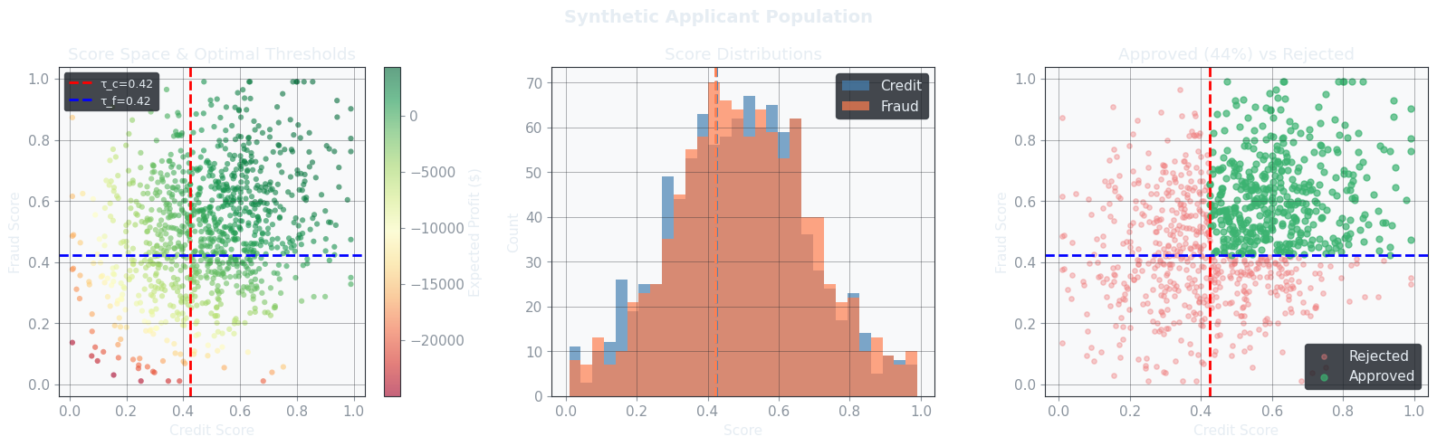
The left scatter plot colors each applicant by their expected individual profit. Applicants in the upper-right quadrant (high credit score, high fraud score) glow green; those near the origin are deep red. The optimal thresholds divide the space into four quadrants; the approved zone is upper-right. The histogram shows both score distributions peaking around 0.5, with the dashed lines marking where the thresholds cut.

Figure 2 — 2D Profit Heatmap:

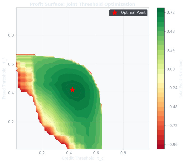
This is the profit surface viewed from directly above. The red star marks the globally optimal $(\tau_c^*, \tau_f^*)$. Notice that the surface is not symmetric: because $L_f > L_d$ (fraud losses exceed credit losses), the contours are more sensitive to $\tau_f$ — moving horizontally (relaxing fraud standards) drops profit faster than moving vertically (relaxing credit standards).

Figure 3 — 3D Profit Surface:

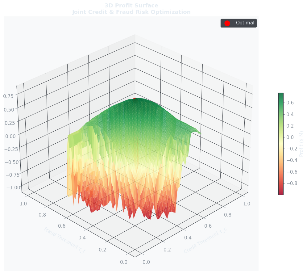
The three-dimensional view reveals the ridge structure. The profit rises as both thresholds increase (stricter screening), but then falls sharply when thresholds are too high (too few applicants approved to generate revenue). The optimal point sits on the shoulder of this ridge — the exact balance between selectivity and volume.

Figure 4 — Lambda Trade-off (four panels):

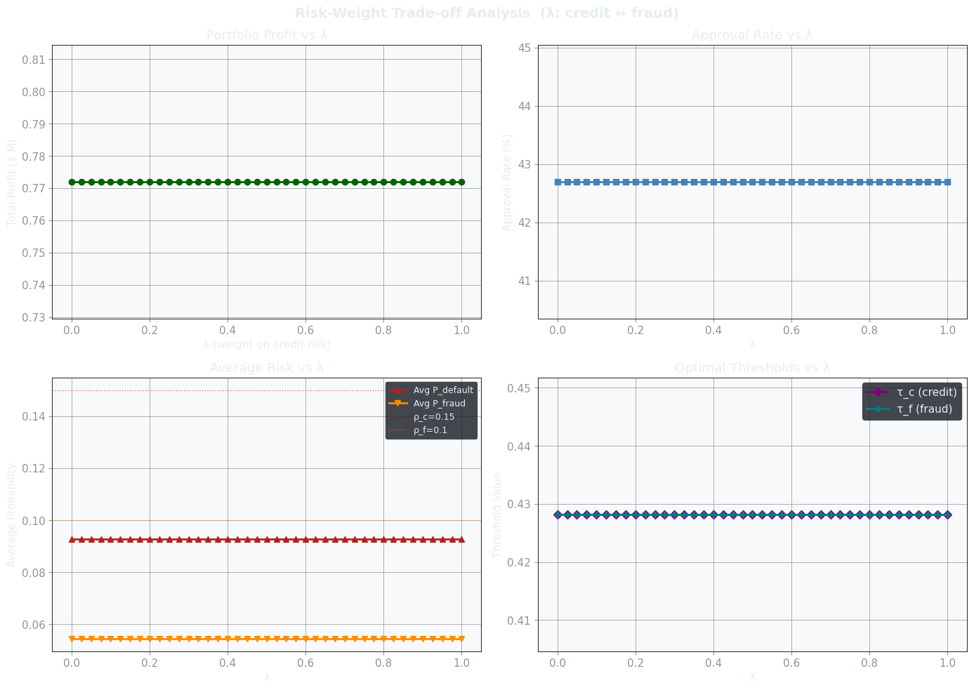
  • Top left: Portfolio profit as a function of $\lambda$. The curve is not monotone — there is a sweet spot.
  • Top right: Approval rate shifts as emphasis moves between risks.
  • Bottom left: Average default and fraud probabilities track the constraints. When $\lambda \approx 0$ (fraud-focused), the bank tightly controls $P_f$ but may allow higher $P_d$.
  • Bottom right: The optimal thresholds $\tau_c, \tau_f$ as $\lambda$ varies — showing how the screening policy adapts.

Figure 5 — 3D Pareto Frontier:

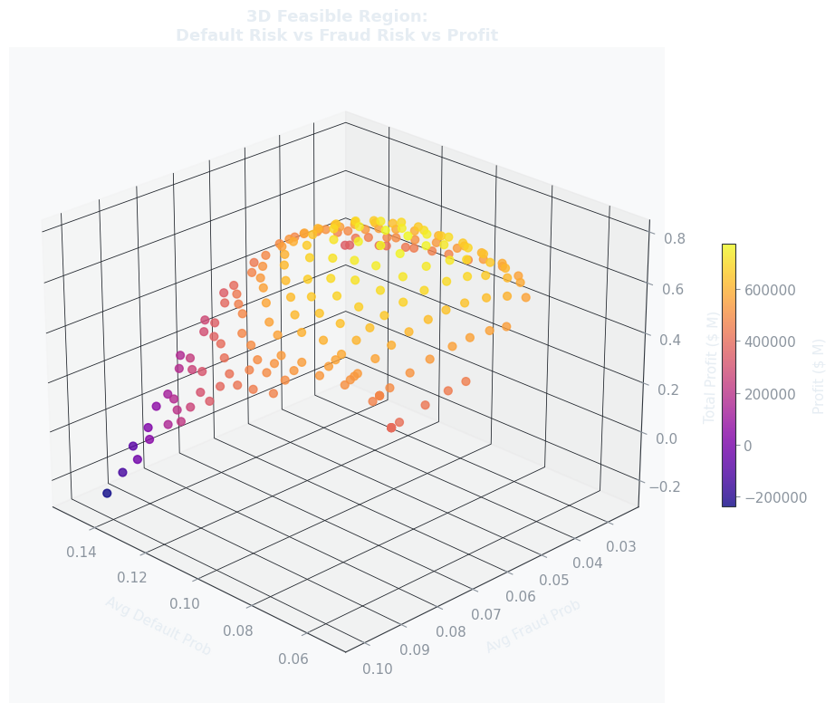
Each point is a feasible threshold pair satisfying all constraints. The x-axis is average default probability, the y-axis is average fraud probability, and the z-axis is total profit. High-profit portfolios cluster in the lower-left corner of the risk plane (low default, low fraud), but reaching them requires increasingly strict thresholds that reduce approval volume — the fundamental three-way tension at the heart of the model.


Key Takeaways

  1. Joint optimization dominates sequential optimization. Setting $\tau_c$ first and $\tau_f$ second (or vice versa) misses interactions between the two risk dimensions.

  2. The profit surface has a well-defined ridge. Being too strict leaves money on the table through rejected good customers; being too lenient generates losses. The optimizer finds the ridge precisely.

  3. $\lambda$ is a management lever, not just a hyperparameter. Shifting $\lambda$ translates directly into different regulatory postures, capital allocations, and approval policies — it should be calibrated against loss data quarterly.

  4. Fraud losses dominate when $L_f > L_d$. In our setup, the optimal $\tau_f^*$ ends up higher than $\tau_c^*$ because the cost of a fraudulent loan exceeds the cost of a defaulted loan. This asymmetry is almost always present in consumer lending.