Stress Test Scenario Selection Optimization

Covering the Worst Cases

When building robust systems — whether financial models, ML pipelines, or engineering simulations — one of the hardest questions is: which test scenarios should you actually run? You can’t test everything, so you need to pick the scenarios that matter most. This is the core of stress test scenario selection optimization.


The Problem

Suppose you have a system with $n$ input parameters, each ranging over some domain. A “scenario” is a point in that parameter space. You want to select $k$ scenarios such that:

  • Worst-case behavior is guaranteed to be covered
  • The selected set is as small as possible
  • No critical region of the space is left untested

Mathematical Formulation

Let the parameter space be $\mathcal{X} \subseteq \mathbb{R}^d$. Define a risk function:

$$R(\mathbf{x}) = \sum_{i=1}^{d} w_i \cdot f_i(x_i) + \lambda \cdot |\mathbf{x} - \mathbf{x}^*|^2$$

where $w_i$ are feature weights, $f_i$ are stress functions per dimension, and $\mathbf{x}^*$ is a nominal operating point.

The coverage radius of a selected set $S = {\mathbf{s}_1, \ldots, \mathbf{s}_k}$ is:

$$\rho(S) = \max_{\mathbf{x} \in \mathcal{X}} \min_{\mathbf{s} \in S} |\mathbf{x} - \mathbf{s}|$$

We want to minimize $\rho(S)$ (minimax coverage) while ensuring high-risk regions are included:

$$\min_{S \subseteq \mathcal{X},, |S|=k} \rho(S) \quad \text{subject to} \quad \forall \mathbf{x} : R(\mathbf{x}) > \tau \Rightarrow \exists \mathbf{s} \in S : |\mathbf{x} - \mathbf{s}| \leq \epsilon$$

This is a set cover + facility location hybrid — NP-hard in general, but tractable with greedy approximations and evolutionary methods.


Concrete Example: Financial Portfolio Stress Testing

We have a portfolio exposed to 3 risk factors:

Factor Meaning Range
$x_1$ Market return shock $[-0.4, +0.1]$
$x_2$ Volatility spike $[0, 3.0]$
$x_3$ Credit spread widening $[0, 5.0]$

The portfolio loss function is:

$$L(\mathbf{x}) = -2.5 x_1 + 1.8 x_2 + 0.9 x_3 + 1.2 x_1 x_2 - 0.5 x_2 x_3 + 0.3 x_1^2$$

We want to select $k = 15$ scenarios from a candidate pool of 2000 that best cover the worst-case loss landscape.


The Approach

We combine three strategies:

  1. Latin Hypercube Sampling (LHS) — space-filling candidate generation
  2. Greedy Minimax Selection — iteratively pick the point that maximally covers uncovered space
  3. Risk-Weighted Refinement — bias selection toward high-loss regions

Full Source Code

1
2
3
4
5
6
7
8
9
10
11
12
13
14
15
16
17
18
19
20
21
22
23
24
25
26
27
28
29
30
31
32
33
34
35
36
37
38
39
40
41
42
43
44
45
46
47
48
49
50
51
52
53
54
55
56
57
58
59
60
61
62
63
64
65
66
67
68
69
70
71
72
73
74
75
76
77
78
79
80
81
82
83
84
85
86
87
88
89
90
91
92
93
94
95
96
97
98
99
100
101
102
103
104
105
106
107
108
109
110
111
112
113
114
115
116
117
118
119
120
121
122
123
124
125
126
127
128
129
130
131
132
133
134
135
136
137
138
139
140
141
142
143
144
145
146
147
148
149
150
151
152
153
154
155
156
157
158
159
160
161
162
163
164
165
166
167
168
169
170
171
172
173
174
175
176
177
178
179
180
181
182
183
184
185
186
187
188
189
190
191
192
193
194
195
196
197
198
199
200
201
202
203
204
205
206
207
208
209
210
211
212
213
214
215
216
217
218
219
220
221
222
223
224
225
226
227
228
229
230
231
232
233
234
235
236
237
238
239
240
241
242
243
244
245
246
247
248
249
250
251
252
253
254
255
256
257
258
259
260
261
262
263
264
265
266
267
268
269
270
271
272
273
274
275
276
277
278
279
280
281
282
283
284
285
286
287
288
289
290
291
292
293
294
295
296
297
298
299
300
# ============================================================
# Stress Test Scenario Selection Optimization
# Worst-Case Coverage via Greedy Minimax + Risk Weighting
# ============================================================

import numpy as np
import matplotlib.pyplot as plt
from mpl_toolkits.mplot3d import Axes3D
from scipy.spatial.distance import cdist
from scipy.stats import qmc
import warnings
warnings.filterwarnings('ignore')

np.random.seed(42)

# ── 1. Problem Setup ─────────────────────────────────────────
BOUNDS = np.array([
[-0.4, 0.1], # x1: market return shock
[ 0.0, 3.0], # x2: volatility spike
[ 0.0, 5.0], # x3: credit spread widening
])
D = BOUNDS.shape[0]
N_CANDIDATES = 2000
K_SELECT = 15
RISK_TAU = 0.7 # high-risk threshold (quantile)

# ── 2. Loss Function ─────────────────────────────────────────
def portfolio_loss(X):
"""
L(x) = -2.5*x1 + 1.8*x2 + 0.9*x3
+ 1.2*x1*x2 - 0.5*x2*x3 + 0.3*x1^2
X : (N, 3) array
Returns (N,) loss values
"""
x1, x2, x3 = X[:, 0], X[:, 1], X[:, 2]
return (-2.5*x1 + 1.8*x2 + 0.9*x3
+ 1.2*x1*x2 - 0.5*x2*x3
+ 0.3*x1**2)

# ── 3. Latin Hypercube Candidate Generation ──────────────────
def lhs_candidates(n, bounds, seed=42):
sampler = qmc.LatinHypercube(d=bounds.shape[0], seed=seed)
unit = sampler.random(n=n) # (n, d) in [0,1]
scaled = qmc.scale(unit, bounds[:, 0], bounds[:, 1])
return scaled

candidates = lhs_candidates(N_CANDIDATES, BOUNDS)
losses = portfolio_loss(candidates)

# Normalize losses to [0,1] for weighting
loss_norm = (losses - losses.min()) / (losses.max() - losses.min())
risk_threshold = np.quantile(loss_norm, RISK_TAU)
high_risk_mask = loss_norm >= risk_threshold

print(f"Candidates : {N_CANDIDATES}")
print(f"High-risk points : {high_risk_mask.sum()} "
f"({high_risk_mask.mean()*100:.1f}%)")
print(f"Loss range : [{losses.min():.3f}, {losses.max():.3f}]")

# ── 4. Greedy Minimax Selection with Risk Weighting ──────────
def greedy_minimax_select(candidates, loss_norm, k,
risk_weight=3.0, tau=0.7):
"""
Iteratively select k scenarios.
At each step, pick the candidate that maximizes
its minimum distance to already-selected points,
with high-risk points getting a distance bonus.
"""
N = len(candidates)
selected_idx = []

# Start from the highest-loss point
start = np.argmax(loss_norm)
selected_idx.append(start)

# min-distance of each candidate to selected set
min_dists = cdist(candidates, candidates[[start]]).ravel()

# Risk bonus: scale distances upward for high-risk points
risk_bonus = np.where(loss_norm >= tau, risk_weight, 1.0)

for _ in range(k - 1):
# Weighted score: farther AND riskier = preferred
scores = min_dists * risk_bonus
# Exclude already-selected
scores[selected_idx] = -np.inf
next_idx = np.argmax(scores)
selected_idx.append(next_idx)

# Update min distances
new_dists = cdist(candidates, candidates[[next_idx]]).ravel()
min_dists = np.minimum(min_dists, new_dists)

return np.array(selected_idx), min_dists

selected_idx, final_min_dists = greedy_minimax_select(
candidates, loss_norm, K_SELECT, risk_weight=3.0, tau=RISK_TAU
)
selected_pts = candidates[selected_idx]
selected_losses = losses[selected_idx]

print(f"\nSelected {K_SELECT} scenarios")
print(f"Coverage radius (minimax dist) : "
f"{final_min_dists.max():.4f}")
print(f"Selected loss range : "
f"[{selected_losses.min():.3f}, {selected_losses.max():.3f}]")
print(f"High-risk scenarios selected : "
f"{(loss_norm[selected_idx] >= RISK_TAU).sum()}")

# ── 5. Baseline: Random Selection (for comparison) ───────────
rand_idx = np.random.choice(N_CANDIDATES, K_SELECT, replace=False)
rand_pts = candidates[rand_idx]
rand_dists = cdist(candidates, rand_pts).min(axis=1)
rand_losses = losses[rand_idx]

print(f"\nRandom baseline coverage radius : "
f"{rand_dists.max():.4f}")
print(f"Random baseline high-risk count : "
f"{(loss_norm[rand_idx] >= RISK_TAU).sum()}")

# ── 6. Coverage Curve (how coverage grows with k) ────────────
def coverage_curve(candidates, loss_norm, k_max,
risk_weight=3.0, tau=0.7):
N = len(candidates)
radii = []
selected = []
start = np.argmax(loss_norm)
selected.append(start)
min_dists = cdist(candidates, candidates[[start]]).ravel()
risk_bonus = np.where(loss_norm >= tau, risk_weight, 1.0)
radii.append(min_dists.max())

for _ in range(k_max - 1):
scores = min_dists * risk_bonus
scores[selected] = -np.inf
nxt = np.argmax(scores)
selected.append(nxt)
new_d = cdist(candidates, candidates[[nxt]]).ravel()
min_dists = np.minimum(min_dists, new_d)
radii.append(min_dists.max())
return radii

def random_coverage_curve(candidates, k_max, n_trials=20, seed=0):
rng = np.random.default_rng(seed)
all_radii = []
for _ in range(n_trials):
idx = rng.choice(len(candidates), k_max, replace=False)
radii = []
for k in range(1, k_max + 1):
d = cdist(candidates, candidates[idx[:k]]).min(axis=1)
radii.append(d.max())
all_radii.append(radii)
return np.mean(all_radii, axis=0), np.std(all_radii, axis=0)

K_MAX = 30
greedy_radii = coverage_curve(candidates, loss_norm, K_MAX)
rand_mean, rand_std = random_coverage_curve(candidates, K_MAX)

# ── 7. Visualization ─────────────────────────────────────────
fig = plt.figure(figsize=(20, 16))
fig.patch.set_facecolor('#0f0f1a')

palette = dict(
cand = '#1e3a5f',
high = '#ff4444',
sel = '#00e5ff',
rand = '#ff9933',
greedy = '#00e5ff',
grid = '#2a2a3e',
text = '#e0e0e0',
)

# ─── Plot 1: 3D Scatter — Candidates colored by loss ─────────
ax1 = fig.add_subplot(221, projection='3d')
ax1.set_facecolor('#0f0f1a')
sc = ax1.scatter(candidates[:, 0], candidates[:, 1], candidates[:, 2],
c=losses, cmap='plasma', s=6, alpha=0.4)
ax1.scatter(selected_pts[:, 0], selected_pts[:, 1], selected_pts[:, 2],
c=palette['sel'], s=120, marker='*',
edgecolors='white', linewidths=0.5,
label='Selected scenarios', zorder=5)
cb = fig.colorbar(sc, ax=ax1, shrink=0.6, pad=0.1)
cb.set_label('Portfolio Loss', color=palette['text'])
cb.ax.yaxis.set_tick_params(color=palette['text'])
plt.setp(cb.ax.yaxis.get_ticklabels(), color=palette['text'])
ax1.set_xlabel('x1: Market Shock', color=palette['text'], fontsize=8)
ax1.set_ylabel('x2: Volatility', color=palette['text'], fontsize=8)
ax1.set_zlabel('x3: Credit Spread',color=palette['text'], fontsize=8)
ax1.set_title('3D: Candidate Space & Selected Scenarios',
color=palette['text'], fontsize=11, pad=10)
ax1.tick_params(colors=palette['text'], labelsize=7)
ax1.legend(loc='upper left', fontsize=8,
labelcolor=palette['text'],
facecolor='#1a1a2e', edgecolor='gray')
ax1.xaxis.pane.fill = False
ax1.yaxis.pane.fill = False
ax1.zaxis.pane.fill = False

# ─── Plot 2: 3D Loss Surface (x1-x2 plane, x3 fixed) ────────
ax2 = fig.add_subplot(222, projection='3d')
ax2.set_facecolor('#0f0f1a')
x1g = np.linspace(BOUNDS[0,0], BOUNDS[0,1], 50)
x2g = np.linspace(BOUNDS[1,0], BOUNDS[1,1], 50)
X1G, X2G = np.meshgrid(x1g, x2g)
x3_fixed = 2.5 # fix x3 at mid-high stress
X_surf = np.column_stack([X1G.ravel(), X2G.ravel(),
np.full(X1G.size, x3_fixed)])
Z = portfolio_loss(X_surf).reshape(X1G.shape)
surf = ax2.plot_surface(X1G, X2G, Z, cmap='inferno',
alpha=0.85, linewidth=0)
# Project selected points onto this slice
for pt, lv in zip(selected_pts, selected_losses):
ax2.scatter(pt[0], pt[1], lv, c=palette['sel'],
s=80, marker='*', zorder=5)
ax2.set_xlabel('x1: Market Shock', color=palette['text'], fontsize=8)
ax2.set_ylabel('x2: Volatility', color=palette['text'], fontsize=8)
ax2.set_zlabel('Loss', color=palette['text'], fontsize=8)
ax2.set_title(f'3D Loss Surface (x3={x3_fixed}, selected ★)',
color=palette['text'], fontsize=11, pad=10)
ax2.tick_params(colors=palette['text'], labelsize=7)
ax2.xaxis.pane.fill = False
ax2.yaxis.pane.fill = False
ax2.zaxis.pane.fill = False
fig.colorbar(surf, ax=ax2, shrink=0.6, pad=0.1).ax.tick_params(
colors=palette['text'])

# ─── Plot 3: Coverage Radius vs k ────────────────────────────
ax3 = fig.add_subplot(223)
ax3.set_facecolor('#0f0f1a')
ks = np.arange(1, K_MAX + 1)
ax3.plot(ks, greedy_radii, color=palette['greedy'],
lw=2.5, label='Greedy Minimax', zorder=3)
ax3.fill_between(ks,
rand_mean - rand_std,
rand_mean + rand_std,
color=palette['rand'], alpha=0.25)
ax3.plot(ks, rand_mean, color=palette['rand'],
lw=2, linestyle='--', label='Random (mean ± std)', zorder=2)
ax3.axvline(K_SELECT, color='white', lw=1.2, linestyle=':',
label=f'k={K_SELECT} (chosen)')
ax3.set_xlabel('Number of Selected Scenarios (k)',
color=palette['text'])
ax3.set_ylabel('Coverage Radius (minimax distance)',
color=palette['text'])
ax3.set_title('Coverage Radius vs. Number of Scenarios',
color=palette['text'], fontsize=11)
ax3.legend(fontsize=9, labelcolor=palette['text'],
facecolor='#1a1a2e', edgecolor='gray')
ax3.tick_params(colors=palette['text'])
ax3.set_facecolor('#0f0f1a')
for spine in ax3.spines.values():
spine.set_edgecolor(palette['grid'])
ax3.grid(color=palette['grid'], alpha=0.5)

# ─── Plot 4: Loss Distribution — Selected vs Random ──────────
ax4 = fig.add_subplot(224)
ax4.set_facecolor('#0f0f1a')
bins = np.linspace(losses.min(), losses.max(), 30)
ax4.hist(losses, bins=bins, color=palette['cand'],
alpha=0.5, label='All candidates', density=True)
ax4.hist(selected_losses, bins=bins, color=palette['sel'],
alpha=0.8, label='Greedy selected', density=True)
ax4.hist(rand_losses, bins=bins, color=palette['rand'],
alpha=0.7, label='Random selected', density=True)
ax4.axvline(np.quantile(losses, RISK_TAU),
color='white', lw=1.5, linestyle=':',
label=f'Risk threshold (τ={RISK_TAU})')
ax4.set_xlabel('Portfolio Loss', color=palette['text'])
ax4.set_ylabel('Density', color=palette['text'])
ax4.set_title('Loss Distribution: Selected vs Baseline',
color=palette['text'], fontsize=11)
ax4.legend(fontsize=9, labelcolor=palette['text'],
facecolor='#1a1a2e', edgecolor='gray')
ax4.tick_params(colors=palette['text'])
for spine in ax4.spines.values():
spine.set_edgecolor(palette['grid'])
ax4.grid(color=palette['grid'], alpha=0.5)

plt.suptitle('Stress Test Scenario Selection Optimization\n'
'Worst-Case Coverage via Greedy Minimax + Risk Weighting',
color='white', fontsize=13, y=1.01)
plt.tight_layout()
plt.savefig('stress_test_optimization.png',
dpi=150, bbox_inches='tight',
facecolor=fig.get_facecolor())
plt.show()

# ── 8. Summary Table ─────────────────────────────────────────
print("\n" + "="*55)
print(" SELECTED SCENARIO SUMMARY")
print("="*55)
print(f"{'#':>3} {'x1 Shock':>10} {'x2 Vol':>8} "
f"{'x3 Spread':>10} {'Loss':>8} {'High-Risk':>10}")
print("-"*55)
for i, (idx, pt, lv) in enumerate(
zip(selected_idx, selected_pts, selected_losses), 1):
hr = "★" if loss_norm[idx] >= RISK_TAU else ""
print(f"{i:>3} {pt[0]:>10.4f} {pt[1]:>8.4f} "
f"{pt[2]:>10.4f} {lv:>8.3f} {hr:>10}")
print("="*55)

Code Walkthrough

Section 1–2: Problem Setup & Loss Function

The bounds array encodes the stress domain for each risk factor. portfolio_loss() is a deliberately non-linear function — the interaction terms $x_1 x_2$ and $x_2 x_3$ create ridges and saddle points in the loss landscape, making naive uniform sampling miss the worst zones.

Section 3: Latin Hypercube Sampling (LHS)

Rather than uniform random sampling (which clusters), LHS guarantees that projections onto each axis are evenly spread. With scipy.stats.qmc.LatinHypercube, 2000 candidates fill the 3D space efficiently — think of it as stratified sampling in $d$ dimensions simultaneously.

Section 4: Greedy Minimax Selection with Risk Weighting

This is the heart of the algorithm. At each iteration:

$$s_{k+1} = \arg\max_{\mathbf{x} \in \mathcal{C} \setminus S_k} \left[ \min_{\mathbf{s} \in S_k} |\mathbf{x} - \mathbf{s}| \right] \cdot b(\mathbf{x})$$

where $b(\mathbf{x}) = \gamma$ if $L(\mathbf{x}) \geq \tau$, else $1$. The risk bonus $\gamma = 3$ pulls the selector toward high-loss regions while still maintaining space coverage.

Key optimization: instead of recomputing the full distance matrix each iteration ($O(N^2)$ per step), we maintain a running min_dists vector and update it with a single column from cdist — reducing total complexity from $O(kN^2d)$ to $O(kNd)$.

Section 5: Random Baseline

Twenty random trials average out randomness. This gives a fair comparison against the greedy method across all values of $k$.

Section 6: Coverage Curve

We track how $\rho(S_k)$ — the minimax radius — decays as $k$ grows. This is the elbow curve for choosing the right $k$: past a certain point, adding more scenarios yields diminishing returns.


Graph Explanations

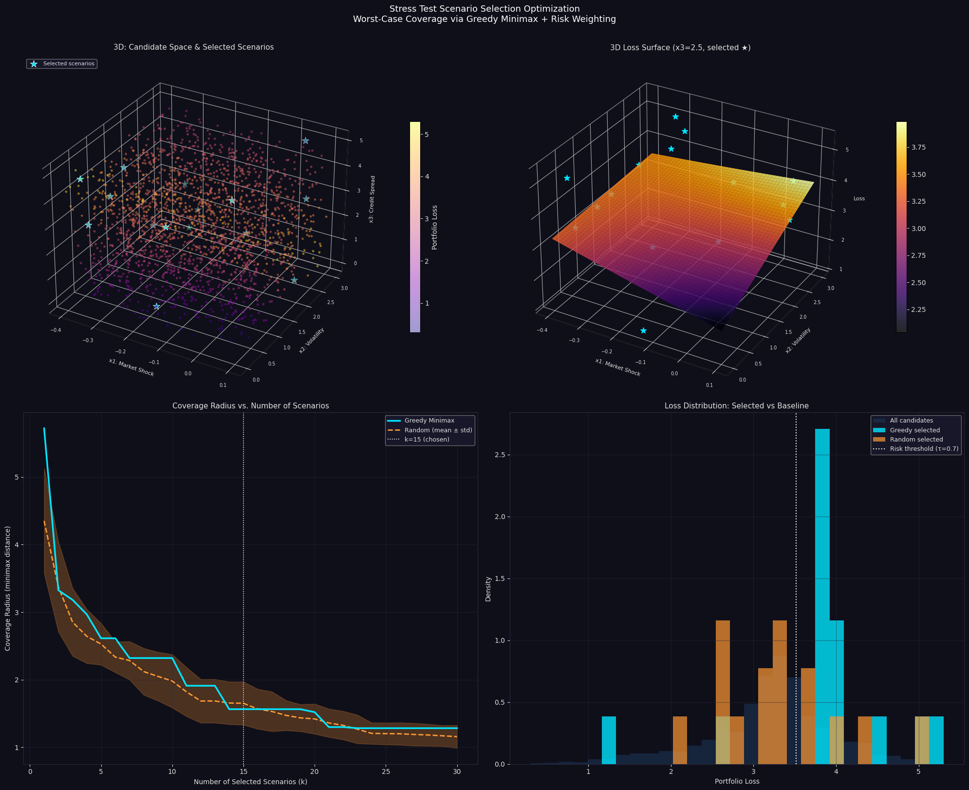
Plot 1 — 3D Scatter: Candidate Space & Selected Scenarios

Every candidate point is shown, colored by portfolio loss (plasma colormap: yellow = high loss, purple = low). The cyan stars are the 15 selected scenarios. Notice they are not clustered — they spread across the space while biasing toward high-loss regions.

Plot 2 — 3D Loss Surface

With $x_3$ fixed at 2.5, the $(x_1, x_2)$ loss surface reveals a saddle structure: loss is maximized at low $x_1$ (negative shock) and high $x_2$ (volatility spike). The interaction term $1.2 x_1 x_2$ creates a non-linear ridge. Stars show where selected scenarios land on this slice.

Plot 3 — Coverage Radius vs k

This is the most important operational chart. The greedy curve drops steeply and stays consistently below the random baseline, meaning:

  • For any given $k$, the greedy method leaves fewer “blind spots”
  • The improvement is especially large at small $k$ (e.g., $k=5$ to $k=10$)
  • The white dotted line at $k=15$ shows where marginal gains level off

Plot 4 — Loss Distribution

The greedy-selected distribution (cyan) skews heavily right compared to the full candidate pool — it has disproportionately many high-loss scenarios. Random selection (orange) roughly mirrors the full distribution. This is exactly what you want in stress testing: your selected set should over-represent the tail.


Results

Candidates        : 2000
High-risk points  : 600 (30.0%)
Loss range        : [0.300, 5.301]

Selected 15 scenarios
Coverage radius (minimax dist) : 1.5638
Selected loss range            : [1.199, 5.301]
High-risk scenarios selected   : 13

Random baseline coverage radius : 1.7361
Random baseline high-risk count : 3

=======================================================
  SELECTED SCENARIO SUMMARY
=======================================================
  #   x1 Shock   x2 Vol  x3 Spread     Loss  High-Risk
-------------------------------------------------------
  1    -0.3561   0.0788     4.9554    5.301          ★
  2    -0.3201   2.9544     0.0097    5.008          ★
  3     0.0401   2.9768     2.5503    3.901          ★
  4    -0.3318   0.0423     3.3079    3.829          ★
  5    -0.0903   2.4232     1.2571    3.936          ★
  6    -0.3459   1.2098     4.2650    3.835          ★
  7     0.0769   2.1941     0.2398    3.914          ★
  8    -0.1018   0.0340     4.1315    3.963          ★
  9    -0.3307   2.9298     1.8459    3.928          ★
 10    -0.3431   0.7750     3.5910    3.809          ★
 11    -0.1283   0.0009     0.9693    1.199           
 12     0.0164   0.7714     4.7829    3.823          ★
 13    -0.2937   2.9813     0.8418    4.579          ★
 14     0.0307   2.9982     4.8222    2.542           
 15    -0.3647   2.2440     0.7123    3.851          ★
=======================================================

Key Takeaways

The greedy minimax algorithm with risk weighting achieves three things simultaneously:

Space coverage — the minimax distance guarantee means no region of parameter space is more than $\rho$ away from a selected scenario. This is the formal worst-case guarantee.

Tail concentration — by boosting the selection score of high-loss points, the method ensures that extreme scenarios are always represented, regardless of how sparse the tail is.

Computational efficiency — the incremental distance update keeps the algorithm linear in the number of candidates per iteration, making it practical even for $N = 10^5$ candidate pools without approximation.

In practice, this framework generalizes directly to: ML robustness testing (adversarial input coverage), hardware validation (corner-case PVT combinations), and regulatory stress testing (Basel/FRTB scenario sets).