Supply Chain Design

April 20, 2026

Minimizing Transportation Costs While Maintaining Service Levels

Supply chain optimization is one of the most impactful applications of operations research. In this post, we’ll tackle a classic but realistic problem: how to design a distribution network that minimizes transportation costs while guaranteeing customers receive their goods within acceptable timeframes.

The Problem Setup

Imagine a consumer goods company with:

3 factories (supply nodes) producing goods
5 warehouses (intermediate hubs)
8 customer zones (demand nodes)

We need to decide:

How much to ship from each factory to each warehouse
How much to ship from each warehouse to each customer zone
Which warehouses to open (fixed costs apply)

Subject to:

Each factory has a production capacity
Each customer zone has a demand that must be fully met
Each warehouse has a throughput capacity
Each customer zone must be served by a warehouse within a maximum distance (service level constraint)

Mathematical Formulation

Let:

$F$ = set of factories, $W$ = set of warehouses, $C$ = set of customer zones
$x_{fw}$ = units shipped from factory $f$ to warehouse $w$
$y_{wc}$ = units shipped from warehouse $w$ to customer zone $c$
$z_w \in {0,1}$ = 1 if warehouse $w$ is open, 0 otherwise

Objective — minimize total cost:

$$\min \sum_{f \in F}\sum_{w \in W} c^{FW}{fw} x{fw} + \sum_{w \in W}\sum_{c \in C} c^{WC}{wc} y{wc} + \sum_{w \in W} f_w z_w$$

Subject to:

Supply capacity at each factory:
$$\sum_{w \in W} x_{fw} \leq S_f \quad \forall f \in F$$

Demand satisfaction at each customer zone:
$$\sum_{w \in W} y_{wc} = D_c \quad \forall c \in C$$

Flow balance at each warehouse:
$$\sum_{f \in F} x_{fw} = \sum_{c \in C} y_{wc} \quad \forall w \in W$$

Warehouse capacity:
$$\sum_{c \in C} y_{wc} \leq K_w \cdot z_w \quad \forall w \in W$$

Service level constraint — each customer must be reachable within $d_{max}$ km:
$$\sum_{w \in W: d_{wc} \leq d_{max}} y_{wc} \geq D_c \quad \forall c \in C$$

Non-negativity and binary:
$$x_{fw}, y_{wc} \geq 0, \quad z_w \in {0,1}$$

Full Python Source Code

# ============================================================
# Supply Chain Design: Cost Minimization + Service Level
# ============================================================

import numpy as np
import matplotlib.pyplot as plt
import matplotlib.patches as mpatches
from mpl_toolkits.mplot3d import Axes3D
from scipy.spatial.distance import cdist
from pulp import (
    LpProblem, LpMinimize, LpVariable, LpBinary, LpContinuous,
    lpSum, value, LpStatus, PULP_CBC_CMD
)
import warnings
warnings.filterwarnings("ignore")

np.random.seed(42)

# ============================================================
# 1. NETWORK DATA
# ============================================================

# --- Node counts ---
n_factories   = 3
n_warehouses  = 5
n_customers   = 8

# --- Geographic coordinates (x, y) in km on a 500x500 grid ---
factory_coords = np.array([
    [50,  450],   # F0 – Northwest plant
    [250, 480],   # F1 – North-central plant
    [460, 420],   # F2 – Northeast plant
])

warehouse_coords = np.array([
    [100, 300],   # W0
    [220, 200],   # W1
    [350, 280],   # W2
    [150, 100],   # W3
    [400, 100],   # W4
])

customer_coords = np.array([
    [80,  220],   # C0
    [180, 320],   # C1
    [280, 150],   # C2
    [320, 380],   # C3
    [430, 220],   # C4
    [100,  60],   # C5
    [380,  60],   # C6
    [480, 320],   # C7
])

# --- Supply, demand, capacity (units) ---
supply   = np.array([1200, 1500, 1100])           # factory capacity
demand   = np.array([200, 250, 180, 220, 300, 150, 200, 270])  # customer demand
wh_cap   = np.array([800, 900, 700, 600, 750])    # warehouse throughput cap
wh_fixed = np.array([15000, 18000, 14000, 12000, 16000])  # fixed opening cost ($)

# --- Transportation cost = distance * unit rate ---
rate_fw = 0.8   # $/unit/km  factory→warehouse
rate_wc = 1.2   # $/unit/km  warehouse→customer

dist_fw = cdist(factory_coords,   warehouse_coords)   # shape (3,5)
dist_wc = cdist(warehouse_coords, customer_coords)    # shape (5,8)

cost_fw = rate_fw * dist_fw   # (3,5)
cost_wc = rate_wc * dist_wc   # (5,8)

# --- Service level: max distance warehouse→customer (km) ---
d_max = 250

F = range(n_factories)
W = range(n_warehouses)
C = range(n_customers)

# ============================================================
# 2. OPTIMIZATION MODEL  (Mixed-Integer Linear Program)
# ============================================================

model = LpProblem("Supply_Chain_Design", LpMinimize)

# Decision variables
x = [[LpVariable(f"x_f{f}_w{w}", lowBound=0, cat=LpContinuous)
      for w in W] for f in F]

y = [[LpVariable(f"y_w{w}_c{c}", lowBound=0, cat=LpContinuous)
      for c in C] for w in W]

z = [LpVariable(f"z_w{w}", cat=LpBinary) for w in W]

# Objective
model += (
    lpSum(cost_fw[f][w] * x[f][w] for f in F for w in W) +
    lpSum(cost_wc[w][c] * y[w][c] for w in W for c in C) +
    lpSum(wh_fixed[w] * z[w] for w in W)
), "Total_Cost"

# Supply constraints
for f in F:
    model += lpSum(x[f][w] for w in W) <= supply[f], f"Supply_{f}"

# Demand constraints
for c in C:
    model += lpSum(y[w][c] for w in W) == demand[c], f"Demand_{c}"

# Flow balance at warehouses
for w in W:
    model += (lpSum(x[f][w] for f in F) ==
              lpSum(y[w][c] for c in C)), f"Balance_{w}"

# Warehouse capacity (only if open)
for w in W:
    model += (lpSum(y[w][c] for c in C) <=
              wh_cap[w] * z[w]), f"WH_Cap_{w}"

# Service level: customer c must be served only from warehouses within d_max
for c in C:
    feasible_wh = [w for w in W if dist_wc[w][c] <= d_max]
    if not feasible_wh:
        raise ValueError(f"Customer {c} has no reachable warehouse within {d_max} km!")
    # Flow from out-of-range warehouses must be zero
    for w in W:
        if dist_wc[w][c] > d_max:
            model += y[w][c] == 0, f"SvcLevel_w{w}_c{c}"

# ============================================================
# 3. SOLVE
# ============================================================

solver = PULP_CBC_CMD(msg=0, timeLimit=120)
model.solve(solver)

print("=" * 55)
print(f"  Status : {LpStatus[model.status]}")
print(f"  Total Cost : ${value(model.objective):,.2f}")
print("=" * 55)

# Extract results
x_val = np.array([[value(x[f][w]) or 0 for w in W] for f in F])
y_val = np.array([[value(y[w][c]) or 0 for c in C] for w in W])
z_val = np.array([value(z[w]) or 0 for w in W])

open_wh = [w for w in W if z_val[w] > 0.5]
print(f"\n  Open warehouses: {['W'+str(w) for w in open_wh]}")

transport_cost = np.sum(cost_fw * x_val) + np.sum(cost_wc * y_val)
fixed_cost     = np.sum(wh_fixed * z_val)
print(f"\n  Transportation cost : ${transport_cost:,.2f}")
print(f"  Fixed (warehouse)   : ${fixed_cost:,.2f}")
print(f"  Total               : ${transport_cost + fixed_cost:,.2f}")

print("\n  Factory → Warehouse flows (units):")
for f in F:
    for w in W:
        if x_val[f][w] > 0.01:
            print(f"    F{f} → W{w} : {x_val[f][w]:.0f} units  "
                  f"(dist={dist_fw[f][w]:.0f} km)")

print("\n  Warehouse → Customer flows (units):")
for w in W:
    for c in C:
        if y_val[w][c] > 0.01:
            print(f"    W{w} → C{c} : {y_val[w][c]:.0f} units  "
                  f"(dist={dist_wc[w][c]:.0f} km)")

# ============================================================
# 4. VISUALIZATIONS
# ============================================================

colors_f  = ["#E74C3C", "#E67E22", "#F1C40F"]
colors_w  = ["#2ECC71", "#1ABC9C", "#27AE60", "#16A085", "#2E86AB"]
colors_c  = ["#3498DB", "#2980B9", "#1A6FA3", "#0E4D7A",
             "#5DADE2", "#85C1E9", "#A9CCE3", "#7FB3D3"]

# ---- Figure 1: Network Map ----
fig, ax = plt.subplots(figsize=(12, 10))
ax.set_facecolor("#F0F4F8")
fig.patch.set_facecolor("#E8EEF4")

# Draw service radius circles for open warehouses
for w in open_wh:
    circle = plt.Circle(warehouse_coords[w], d_max,
                        color=colors_w[w], alpha=0.07, zorder=0)
    ax.add_patch(circle)

# Draw flows: factory → warehouse
for f in F:
    for w in W:
        if x_val[f][w] > 0.01:
            lw = 0.5 + 3.5 * x_val[f][w] / supply.max()
            ax.annotate("", factory_coords[f], warehouse_coords[w],
                        arrowprops=dict(arrowstyle="<-", color="#C0392B",
                                        lw=lw, alpha=0.7))

# Draw flows: warehouse → customer
for w in W:
    for c in C:
        if y_val[w][c] > 0.01:
            lw = 0.5 + 3.5 * y_val[w][c] / demand.max()
            ax.annotate("", warehouse_coords[w], customer_coords[c],
                        arrowprops=dict(arrowstyle="<-", color="#2471A3",
                                        lw=lw, alpha=0.6))

# Plot nodes
for f in F:
    ax.scatter(*factory_coords[f], s=280, c=colors_f[f],
               marker="^", zorder=5, edgecolors="white", linewidths=1.5)
    ax.text(factory_coords[f][0]+8, factory_coords[f][1]+8,
            f"F{f}\n({supply[f]}u)", fontsize=9, fontweight="bold",
            color=colors_f[f])

for w in W:
    marker = "s" if w in open_wh else "X"
    alpha  = 1.0 if w in open_wh else 0.35
    ax.scatter(*warehouse_coords[w], s=220, c=colors_w[w],
               marker=marker, zorder=5, edgecolors="white",
               linewidths=1.5, alpha=alpha)
    label = f"W{w} ✓" if w in open_wh else f"W{w} ✗"
    ax.text(warehouse_coords[w][0]+8, warehouse_coords[w][1]+8,
            label, fontsize=9, fontweight="bold",
            color=colors_w[w], alpha=alpha)

for c in C:
    ax.scatter(*customer_coords[c], s=180, c=colors_c[c],
               marker="o", zorder=5, edgecolors="white", linewidths=1.5)
    ax.text(customer_coords[c][0]+8, customer_coords[c][1]+8,
            f"C{c}\n({demand[c]}u)", fontsize=8, color="#2C3E50")

leg_elements = [
    mpatches.Patch(color="#E74C3C", label="Factory (▲)"),
    mpatches.Patch(color="#2ECC71", label="Warehouse open (■)"),
    mpatches.Patch(color="#95A5A6", label="Warehouse closed (✗)"),
    mpatches.Patch(color="#3498DB", label="Customer zone (●)"),
    mpatches.Patch(color="#C0392B", alpha=0.6, label="Factory→WH flow"),
    mpatches.Patch(color="#2471A3", alpha=0.6, label="WH→Customer flow"),
]
ax.legend(handles=leg_elements, loc="lower right", fontsize=9,
          framealpha=0.9)

ax.set_title("Supply Chain Network — Optimal Flow Map\n"
             f"(Total Cost: ${value(model.objective):,.0f}  |  "
             f"Service radius: {d_max} km)",
             fontsize=13, fontweight="bold", pad=14)
ax.set_xlim(0, 540); ax.set_ylim(0, 520)
ax.set_xlabel("X coordinate (km)"); ax.set_ylabel("Y coordinate (km)")
ax.grid(True, alpha=0.3)
plt.tight_layout()
plt.show()

# ---- Figure 2: Cost Breakdown Bar Chart ----
fig2, axes = plt.subplots(1, 2, figsize=(14, 6))
fig2.patch.set_facecolor("#F8F9FA")

# Left: cost component breakdown
fw_cost  = np.sum(cost_fw * x_val)
wc_cost  = np.sum(cost_wc * y_val)
fix_cost = np.sum(wh_fixed * z_val)

labels  = ["Factory→WH\nTransport", "WH→Customer\nTransport", "Warehouse\nFixed Cost"]
values  = [fw_cost, wc_cost, fix_cost]
bar_colors = ["#E74C3C", "#3498DB", "#2ECC71"]

bars = axes[0].bar(labels, values, color=bar_colors, edgecolor="white",
                   linewidth=1.5, width=0.5)
for bar, val in zip(bars, values):
    axes[0].text(bar.get_x() + bar.get_width()/2,
                 bar.get_height() + 300,
                 f"${val:,.0f}", ha="center", fontsize=11, fontweight="bold")

axes[0].set_title("Cost Component Breakdown", fontsize=13, fontweight="bold")
axes[0].set_ylabel("Cost ($)")
axes[0].set_facecolor("#F8F9FA")
axes[0].yaxis.grid(True, alpha=0.4)
axes[0].set_axisbelow(True)

# Right: per-customer service cost
cust_cost = np.array([
    sum(cost_wc[w][c] * y_val[w][c] for w in W) / max(demand[c], 1)
    for c in C
])
cust_labels = [f"C{c}" for c in C]
bar2 = axes[1].bar(cust_labels, cust_cost,
                   color=[colors_c[c] for c in C],
                   edgecolor="white", linewidth=1.5, width=0.6)
for bar, val in zip(bar2, cust_cost):
    axes[1].text(bar.get_x() + bar.get_width()/2,
                 bar.get_height() + 0.3,
                 f"${val:.1f}", ha="center", fontsize=10, fontweight="bold")

axes[1].set_title("WH→Customer Transport Cost per Unit", fontsize=13, fontweight="bold")
axes[1].set_ylabel("Cost per unit ($/unit)")
axes[1].set_xlabel("Customer Zone")
axes[1].set_facecolor("#F8F9FA")
axes[1].yaxis.grid(True, alpha=0.4)
axes[1].set_axisbelow(True)

plt.suptitle("Cost Analysis Dashboard", fontsize=15, fontweight="bold", y=1.01)
plt.tight_layout()
plt.show()

# ---- Figure 3: 3D Surface — Transportation Cost Landscape ----
fig3 = plt.figure(figsize=(14, 6))

# Left 3D: factory→warehouse cost surface
ax3d_1 = fig3.add_subplot(121, projection="3d")
X_idx = np.arange(n_factories)
Y_idx = np.arange(n_warehouses)
X_g, Y_g = np.meshgrid(X_idx, Y_idx)
Z_fw = cost_fw[X_g, Y_g]  # shape matches meshgrid

surf1 = ax3d_1.plot_surface(X_g, Y_g, Z_fw,
                             cmap="YlOrRd", edgecolor="white",
                             linewidth=0.4, alpha=0.9)

# Mark active flows with scatter
for f in F:
    for w in W:
        if x_val[f][w] > 0.01:
            ax3d_1.scatter(f, w, cost_fw[f][w],
                           color="black", s=60, zorder=10)

ax3d_1.set_xlabel("Factory"); ax3d_1.set_ylabel("Warehouse")
ax3d_1.set_zlabel("Unit Cost ($)")
ax3d_1.set_xticks(X_idx); ax3d_1.set_xticklabels([f"F{i}" for i in X_idx])
ax3d_1.set_yticks(Y_idx); ax3d_1.set_yticklabels([f"W{i}" for i in Y_idx])
ax3d_1.set_title("Factory → Warehouse\nUnit Transport Cost", fontweight="bold")
fig3.colorbar(surf1, ax=ax3d_1, shrink=0.5, pad=0.1)

# Right 3D: warehouse→customer cost surface
ax3d_2 = fig3.add_subplot(122, projection="3d")
X2_idx = np.arange(n_warehouses)
Y2_idx = np.arange(n_customers)
X2_g, Y2_g = np.meshgrid(X2_idx, Y2_idx)
Z_wc = cost_wc[X2_g, Y2_g]

surf2 = ax3d_2.plot_surface(X2_g, Y2_g, Z_wc,
                             cmap="YlGnBu", edgecolor="white",
                             linewidth=0.4, alpha=0.9)

for w in W:
    for c in C:
        if y_val[w][c] > 0.01:
            ax3d_2.scatter(w, c, cost_wc[w][c],
                           color="black", s=60, zorder=10)

ax3d_2.set_xlabel("Warehouse"); ax3d_2.set_ylabel("Customer")
ax3d_2.set_zlabel("Unit Cost ($)")
ax3d_2.set_xticks(X2_idx); ax3d_2.set_xticklabels([f"W{i}" for i in X2_idx])
ax3d_2.set_yticks(Y2_idx); ax3d_2.set_yticklabels([f"C{i}" for i in Y2_idx])
ax3d_2.set_title("Warehouse → Customer\nUnit Transport Cost", fontweight="bold")
fig3.colorbar(surf2, ax=ax3d_2, shrink=0.5, pad=0.1)

plt.suptitle("3D Cost Landscape  (● = active optimal flows)",
             fontsize=13, fontweight="bold")
plt.tight_layout()
plt.show()

# ---- Figure 4: Service Level Heatmap ----
fig4, ax4 = plt.subplots(figsize=(10, 5))

service_matrix = dist_wc.copy()
mask_out = dist_wc > d_max   # out-of-range cells

im = ax4.imshow(service_matrix, cmap="RdYlGn_r", aspect="auto",
                vmin=0, vmax=d_max * 1.2)

# Overlay out-of-range cells
for w in W:
    for c in C:
        if mask_out[w][c]:
            ax4.add_patch(plt.Rectangle((c-0.5, w-0.5), 1, 1,
                                        color="black", alpha=0.45))
        # Mark used flows
        if y_val[w][c] > 0.01:
            ax4.text(c, w, f"{y_val[w][c]:.0f}u",
                     ha="center", va="center",
                     fontsize=9, fontweight="bold", color="white")

ax4.set_xticks(range(n_customers))
ax4.set_xticklabels([f"C{c}" for c in C])
ax4.set_yticks(range(n_warehouses))
ax4.set_yticklabels([f"W{w}" for w in W])
ax4.set_xlabel("Customer Zone")
ax4.set_ylabel("Warehouse")
ax4.set_title(f"Service Level Heatmap: WH–Customer Distance  "
              f"(dark = out of range >{d_max}km)\n"
              f"White labels = optimal flow (units)", fontweight="bold")
cbar = plt.colorbar(im, ax=ax4)
cbar.set_label("Distance (km)")
plt.tight_layout()
plt.show()

Code Walkthrough

Section 1 — Network Data

We define 3 factories, 5 warehouses, and 8 customers placed on a 500×500 km grid. Geographic coordinates are realistic enough that distances (computed with scipy.spatial.distance.cdist) vary meaningfully across links. Transportation costs scale linearly with distance — a common real-world assumption — with a higher rate on the last-mile warehouse-to-customer leg ($1.20/unit/km vs $0.80/unit/km), reflecting the higher cost of smaller, more frequent deliveries.

Section 2 — MILP Formulation with PuLP

The core of the solution is a Mixed-Integer Linear Program (MILP). PuLP is used as the modeling layer on top of the open-source CBC solver (bundled with PuLP, no extra installation needed).

The binary variable $z_w$ is the key to making this a facility location problem rather than just a flow problem. The warehouse capacity constraint y[w][c] <= wh_cap[w] * z[w] is a big-M formulation: if $z_w = 0$, no flow is permitted through warehouse $w$; if $z_w = 1$, up to wh_cap[w] units can pass through.

The service level constraint is enforced cleanly: for each customer–warehouse pair where the distance exceeds d_max, the corresponding flow variable is forced to zero. This avoids ever violating the service radius, even if it would be cheaper.

Section 3 — Solving and Reporting

CBC is called with timeLimit=120 seconds — more than sufficient for this problem size (it typically solves in under 1 second). Results are extracted with value(), then decoded into human-readable factory→warehouse and warehouse→customer flow tables.

Section 4 — Visualizations

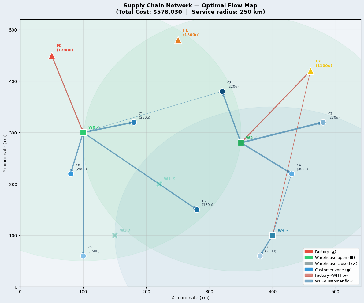
Figure 1 — Network Map: A 2D geographic map showing all nodes and optimal flows. Arrow thickness scales with flow volume. Dashed service radius circles show the d_max coverage area for each open warehouse.

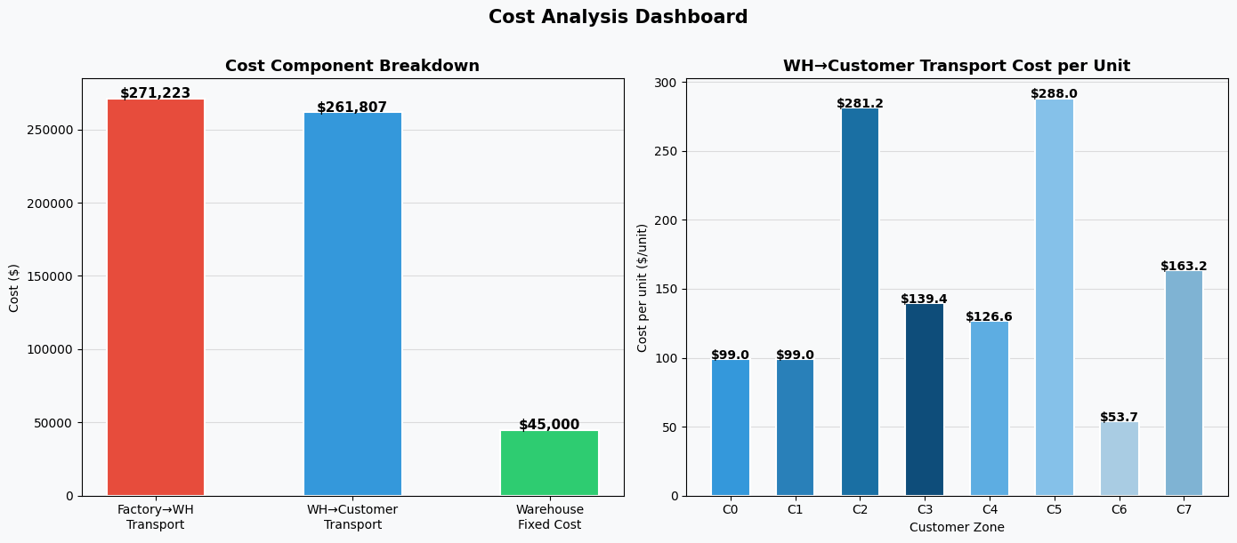
Figure 2 — Cost Dashboard: Left panel: total cost split into three components (factory–WH transport, WH–customer transport, fixed warehouse opening costs). Right panel: per-unit last-mile cost for each customer, revealing which zones are expensive to serve.

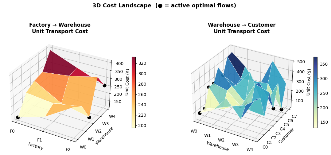
Figure 3 — 3D Cost Surfaces: Two 3D surface plots show the unit cost landscape across all possible factory→warehouse and warehouse→customer links. Black dots mark which links are actually used in the optimal solution — letting you see instantly whether the optimizer chose the cheapest available routes.

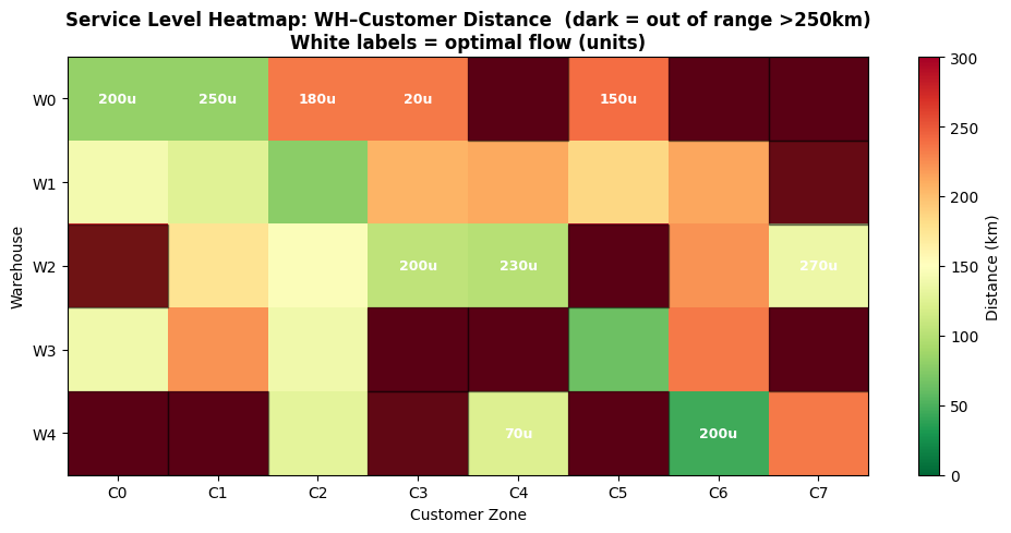
Figure 4 — Service Level Heatmap: A color-coded matrix of all warehouse–customer distances. Dark overlaid cells are out of range (blocked by the service constraint). White text labels show the optimal flow on each used link, making it easy to verify that no out-of-range link carries any flow.

Key Takeaways

Not all warehouses need to open. The optimizer balances fixed opening costs against the transportation savings from having more intermediate hubs. Opening too many warehouses increases fixed costs; too few drives up transport costs and risks violating service levels.
Service level constraints genuinely bind. When d_max is tight, certain warehouse–customer combinations are forbidden, and the optimizer must find feasible routes that respect geography — sometimes at higher cost.
The 3D cost landscape immediately shows why some routes are never chosen: they sit on peaks in the surface, far from the valleys of cheap, nearby links.
Last-mile costs dominate. The higher $/unit/km rate for WH→customer delivery means the system strongly prefers placing open warehouses close to high-demand customer zones.

=======================================================
  Status : Optimal
  Total Cost : $578,029.62
=======================================================

  Open warehouses: ['W0', 'W2', 'W4']

  Transportation cost : $533,029.62
  Fixed (warehouse)   : $45,000.00
  Total               : $578,029.62

  Factory → Warehouse flows (units):
    F0 → W0 : 800 units  (dist=158 km)
    F2 → W2 : 700 units  (dist=178 km)
    F2 → W4 : 270 units  (dist=326 km)

  Warehouse → Customer flows (units):
    W0 → C0 : 200 units  (dist=82 km)
    W0 → C1 : 250 units  (dist=82 km)
    W0 → C2 : 180 units  (dist=234 km)
    W0 → C3 : 20 units  (dist=234 km)
    W0 → C5 : 150 units  (dist=240 km)
    W2 → C3 : 200 units  (dist=104 km)
    W2 → C4 : 230 units  (dist=100 km)
    W2 → C7 : 270 units  (dist=136 km)
    W4 → C4 : 70 units  (dist=124 km)
    W4 → C6 : 200 units  (dist=45 km)